On some new travelling wave structures to the (3+1)-dimensional Boiti-Leon-Manna-Pempinelli model

Kalim U. Tariq; Ahmet Bekir; Muhammad Zubair

doi:10.1016/j.joes.2022.03.015

Journal of Ocean Engineering and Science >

2024 , Vol. 9 >Issue 2: 99 - 111

DOI: https://doi.org/10.1016/j.joes.2022.03.015

Research article

On some new travelling wave structures to the (3+1)-dimensional Boiti-Leon-Manna-Pempinelli model

Kalim U. Tariq ^,^a ,
Ahmet Bekir ^,^b^,^* ,
Muhammad Zubair ^a

Expand

^a Department of Mathematics, Mirpur University of Science and Technology, Mirpur 10250 AJK, Pakistan
^b Neighbourhood of Akcaglan, Imarli Street, Number: 28/4, Eskisehir, 26030 Turkey

^*E-mail addresses: kalimulhaq@must.edu.pk (K.U. Tariq),

bekirahmet@gmail.com(A. Bekir).

Received date: 2022-01-12

Revised date: 2022-03-15

Accepted date: 2022-03-15

Online published: 2022-03-21

Fold

Abstract

In this article, the (1Gâ€²) -expansion method, the Bernoulli sub-ordinary differential equation method and the modified Kudryashov method are implemented to construct a variety of novel analytical solutions to the (3+1)-dimensional Boiti-Leon-Manna-Pempinelli model representing the wave propagation through incompressible fluids. The linearization of the wave structure in shallow water necessitates more critical wave capacity conditions than it does in deep water, and the strong nonlinear properties are perceptible. Some novel travelling wave solutions have been observed including solitons, kink, periodic and rational solutions with the aid of the latest computing tools such as Mathematica or Maple. The physical and analytical properties of several families of closed-form solutions or exact solutions and rational form function solutions to the (3+1)-dimensional Boiti-Leon-Manna-Pempinelli model problem are examined using Mathematica.

Highlights

● The study of nonlinear wave structures is becoming one of the dominant disciplines in diverse fields of nonlinear sciences, such ocean physics, fluid dynamics, hydrodynamics, marine engineering.

● This model has been widely used in various complicated travelling interface problems in materials science and fluid dynamics through a phase-field approach.

● A variety of solitons are observed namely, bright, dark, singular, combo, optical, singular optical and bright-singular combo soliton solutions are demonstrated.

● The acquired solutions alongside particular values of involved free parameters are figured out in 3D, 2D and contour profiles to depict diverse soliton patterns.

Key words： The (3+1)-dimensional; Boiti-Leon-Manna-Pempinelli model; The ($\frac{1}{G'}$) -expansion method; The Bernoulli sub-ODE method; The modified Kudryashov method

Cite this article

Kalim U. Tariq , Ahmet Bekir , Muhammad Zubair . On some new travelling wave structures to the (3+1)-dimensional Boiti-Leon-Manna-Pempinelli model[J]. Journal of Ocean Engineering and Science, 2024 , 9(2) : 99 -111 . DOI: 10.1016/j.joes.2022.03.015

1. Introduction

In the study of nonlinear physical phenomenon, the exploration of soliton wave solutions posses nonlinear evolution equations (NLEEs) is crucial. In the last several decades, this field had been researched. The study of nonlinear wave structures is becoming one of the dominant disciplines to describe nonlinear complex phenomena in diverse fields of nonlinear sciences, such as plasma physics, ocean physics, fluid dynamics, hydrodynamics, marine engineering, and many more [1], [2], [3], [4], [5], [6], [7], [8], [9].

Based on developments in computing tools, investigations of the exact solutions of those equations are currently rather spectacular. The Jacobi elliptic function expansion method [10], [11], the Exp-function method [12], the F-expansion method [13], the sub-ODE method [14], the parameter-expansion method [15], the lie symmetry analysis [11], the inverse scattering method [16], the variational iteration method [17], the tanh-method [18], the extended sinh-Gordon equation expansion method [19], the extended tanh-method [20], the homogeneous balance method [21], the extended truncated expansion approach, the Adomian decomposition method [22] and the homotopy perturbation method [23] are few approaches to understand the behaviour of various interesting nonlinear wave structures of recent era [24], [25], [26].

Some new travelling wave solutions have been computed including singular solitons, kink shaped and periodic solutions with the aid of the new computing tools such as Mathematica. In the Soliton theory, the solitary wave solutions interact with one other without losing amplitude or velocity. Their identities and forms, for example, do not change as a result of their reciprocal interactions. Furthermore, the newly developed solutions and their graphical representations demonstrate various dynamical patterns of solitary waves, which is critical to develop a pre-eminent understanding about NLEEs emerging in diverse disciplines of science and engineering [27], [28], [29], [30], [31], [32], [33], [34], [35], [36], [37].

Darvishi et al. introduced a well known model of ocean engineering namely the (3+1)-dimensional Boiti-Leon-Manna-Pempinelli (BLMP) model in 2012 [38], which describes the evolution of the horizontal velocity component of water waves propagating in the xy-plane in an infinite narrow channel of constant depth and can be considered as a model for incompressible fluid as an extension of the (2+1)-dimensional BLMP equation. X. Y. Gao studied the shock wave behaviour of this model by using the auto-Bäcklund transformation [39] while Li et al, employed the Bilinear method is used to develop some interesting forms of multiple-lump waves, namely, two-, four- and eight-lump waves, ump waves, breather waves, mixed waves, and multi-soliton wave solutions [40], later A. M. Wazwaz applied the simplified Hirota's method to deal the newly constructed models with constant coefficients and time-dependent coefficients. For obtaining multiple complicated soliton solutions, the author also employs the complex Hirota's criteria [41].

The aim of the study is to attain the exact solutions to the 3-dimensional BLMP model by employing the the

(\frac{1}{G^{'}})

-expansion approach and the Bernoulli sub-ODE approach and the modified Kudryashov method. The governing reads [42]

(1)

- 3 u_{x} (u_{x y} + u_{x z}) - 3 u_{x x} (u_{y} + u_{z}) + u_{x x x y} u_{x x x z} + u_{y t} + u_{z t} = 0,

which describes the motion of antiphase boundaries in crystalline solids and has been widely used in various complicated travelling interface problems in materials science and fluid dynamics through a phase-field approach [43].

In this article, the produced closed-form solitary wave solutions are stated in terms of hyperbolic, trigonometric, and exponential rational functions with arbitrary constants.

2. Methodology

2.1. The Bernoulli sub-ode method

Consider the NLEE of the form:

(2)

G (u, u_{x}, u_{t}, u_{x x}, u_{x t}, u_{t t}, \dots) = 0,

where

u = u (x, t)

is the unknown function and

G

is a polynomial.

Consider the transformation

U (ξ) = u (x, t),

where

ξ = k (x - c t),

where

ω

is constant speed of wave. After using this transformation the above NLPDE convert into the following nonlinear ODE

(3)

G (u, u^{'}, u^{″}, u^{″'}, \dots) = 0,

the solution of the Eq. (2) is of the form

(4)

u (ξ) = a_{0} + \sum_{i = 1}^{m} a_{i} {(G)}^{i},

where

a_{i}

i = 1, 2, 3, \dots, m

are the constants to computed and

m

is calculated by homogenous balance principle by comparing the highest order derivative and the highest degree of nonlinear term and

G = G (ξ)

provides the following second order ODE

(5)

G^{'} (ξ) + λ G (ξ) = μ G {(ξ)}^{2},

where

λ

and

μ

are constants and

(6)

G (ξ) = \frac{1}{d e^{λ ξ} + \frac{μ}{λ}},

The required derivatives of Eq. (4) are determined and putting in Eq. (3) and collecting the coefficients of

(\frac{1}{G})

by setting of coefficients of polynomial to zero, an algebraic equation system is produced. These models are solved by Mathematica 11.0 program and substitute in Eq. (2) the solutions of Eq. (1) are obtained.

2.2. The $(\frac{1}{G^{'}})$ -expansion method

Consider the NLPDE of the form:

(7)

G (u, u_{x}, u_{t}, u_{x x}, u_{x t}, u_{t t}, \dots) = 0,

where

u = u (x, t)

is the unknown function and

G

is a polynomial.

Consider the transformation

U (ξ) = u (x, t),

and

ξ = x - ω t,

for

ω \neq 0

, where

ω

is constant speed of wave. After using this transformation the above NLPDE convert into the following nonlinear ODE

(8)

G (u, u^{'}, u^{″}, u^{″'}, \dots) = 0,

the solution of the Eq. (8) is of the form

(9)

u (ξ) = a_{0} + \sum_{i = 1}^{m} a_{i} {(\frac{1}{G^{'}})}^{i},

where

a_{i}

i = 1, 2, 3, \dots, m

are the constants to computed and

m

is calculated by homogenous balance principle by comparing the highest order derivative and the highest degree of nonlinear term and

G = G (ξ)

provides the following second order ODE

(10)

G^{″} + λ G^{'} + μ = 0,

where

λ

and

μ

are constants and

(11)

\frac{1}{G^{'}} = \frac{λ}{A λ (\cosh (λ ξ) - \sinh (λ ξ)) - μ},

where A is an integral constant. The required derivatives of Eq. (9) are determined and putting in Eq. (8) and collecting the coefficients of

(\frac{1}{G^{'}})

by setting of coefficients of polynomial to zero, an algebraic equation system is produced. These models are solved by Mathematica 11.0 program and substitute in Eq. (7) the solutions of Eq. (1) are obtained.

2.3. The modified Kudryashov method

Consider the NLPDE of the form:

(12)

G (u, u_{x}, u_{t}, u_{x x}, u_{x t}, u_{t t}, \dots) = 0,

where

u = u (x, t)

is the unknown function and

G

is a polynomial.

Using the transformation

u (x, t) = U (ξ)

where

ξ = κ x + ω t

varies according to given equation, this will carries the Eq. (12) to the nonlinear ODE of the form

(13)

H (U, U^{'}, U^{″}, \dots) = 0,

H

is the polynomial in

U

and the derivatives are ordinary with respect to

ξ

Suppose the solution of Eq. (13) is of the form

(14)

U (ξ) = a_{0} + \sum_{j = 1}^{N} a_{j} Q^{j} (ξ), a_{N} \neq 0,

where the constants

a_{j}

(j = 0, 1, \dots, N)

will be determine and positive integer

N

is calculated by balancing principle.

Q (ξ)

satisfies the ode

(15)

Q^{'} (ξ) = (Q^{2} (ξ) - Q (ξ)) ln (A),

where

Q (ξ) = \frac{1}{{dA}^{ξ} + 1}

, and

A \neq 0, 1

Susbtituting Eq. (14) in Eq. (13) and using mathematical teachnique we obtained a set of algebraic equations in parameters

a_{j}

(j = 0, 1, \dots, N)

k

and

ω

. Finally obtained new exact solutions for the Eq. (1) by arranging the extracted values in Eq. (13)

3. Mathematical analysis

Consider transformation

(16)

u (x, y, z, t) = ζ (X),

where

X = κ x + δ y + γ z + t v,

Equation (1) reduces to

(17)

κ^{3} ζ^{4} - 6 κ^{2} ζ^{'} ζ^{″} + v ζ^{″} = 0

3.1. Applications to the Bernouli sub-ode method

By balancing principle we achieve

N = 1

. The solution of Eq. (1) of form

(18)

u (X) = b_{1} G (X) + b_{0},

satisfies the above equation

\begin{matrix} G^{'} (X) + λ G (X) = μ G {(X)}^{2}, \end{matrix}

\begin{matrix} G (X) = \frac{1}{d e^{λ X} + \frac{μ}{λ}}, \end{matrix}

putting Eq. (18) along with its first two derivative and collecting coefficient of

\frac{1}{G (η)}

, we obtained following system:

\begin{matrix} b_{1} κ^{3} λ^{4} + b_{1} λ^{2} v = 0, \\ - 15 b_{1} κ^{3} λ^{3} μ + 6 b_{1}^{2} κ^{2} λ^{3} - 3 b_{1} λ μ v = 0, \\ 50 b_{1} κ^{3} λ^{2} μ^{2} - 24 b_{1}^{2} κ^{2} λ^{2} μ + 2 b_{1} μ^{2} v = 0, \\ 30 b_{1}^{2} κ^{2} λ μ^{2} - 60 b_{1} κ^{3} λ μ^{3} = 0, \\ 24 b_{1} κ^{3} μ^{4} - 12 b_{1}^{2} κ^{2} μ^{3} = 0 . \end{matrix}

Family I.

Case I.

\begin{matrix} b_{1} = 2 κ μ, λ = - \frac{i \sqrt{v}}{κ^{3 / 2}}, \end{matrix}

\begin{matrix} u_{1} (x, y, z, t) & = & b_{0} + \frac{2 κ μ}{d \exp (- \frac{i \sqrt{v} (t v - \frac{i \sqrt{v} z}{κ^{3 / 2}} + κ x + μ y)}{κ^{3 / 2}}) + \frac{i κ^{3 / 2} μ}{\sqrt{v}}} . \end{matrix}

Case II.

\begin{matrix} b_{1} = 2 κ μ, λ = \frac{i \sqrt{v}}{κ^{3 / 2}}, \end{matrix}

\begin{matrix} u_{2} (x, y, z, t) & = & b_{0} + \frac{2 κ μ}{d \exp (\frac{i \sqrt{v} (t v + \frac{i \sqrt{v} z}{κ^{3 / 2}} + κ x + μ y)}{κ^{3 / 2}}) - \frac{i κ^{3 / 2} μ}{\sqrt{v}}} . \end{matrix}

Family II.

Case I.

\begin{matrix} κ = - \frac{\sqrt[3]{v}}{λ^{2 / 3}}, b_{1} = - \frac{2 μ \sqrt[3]{v}}{λ^{2 / 3}}, \end{matrix}

\begin{matrix} u_{3} (x, y, z, t) & = & b_{0} - \frac{2 \sqrt[3]{λ} μ \sqrt[3]{v}}{d λ e^{λ (t v - \frac{\sqrt[3]{v} x}{λ^{2 / 3}} + μ y + λ z)} + μ} . \end{matrix}

Case II.

\begin{matrix} κ = \frac{\sqrt[3]{- 1} \sqrt[3]{v}}{λ^{2 / 3}}, b_{1} = \frac{2 \sqrt[3]{- 1} μ \sqrt[3]{v}}{λ^{2 / 3}}, \end{matrix}

\begin{matrix} u_{4} (x, y, z, t) & = & b_{0} + \frac{2 \sqrt[3]{- 1} \sqrt[3]{λ} μ \sqrt[3]{v}}{d λ e^{λ (t v + \frac{\sqrt[3]{- 1} \sqrt[3]{v} x}{λ^{2 / 3}} + μ y + λ z)} + μ} . \end{matrix}

Case III.

\begin{matrix} κ = - \frac{{(- 1)}^{2 / 3} \sqrt[3]{v}}{λ^{2 / 3}}, b_{1} = - \frac{2 {(- 1)}^{2 / 3} μ \sqrt[3]{v}}{λ^{2 / 3}}, \end{matrix}

\begin{matrix} u_{5} (x, y, z, t) & = & b_{0} - \frac{2 {(- 1)}^{2 / 3} \sqrt[3]{λ} μ \sqrt[3]{v}}{d λ \exp (λ (t v - \frac{{(- 1)}^{2 / 3} \sqrt[3]{v} x}{λ^{2 / 3}} + μ y + λ z)) + μ} . \end{matrix}

Family III.

Case I.

\begin{matrix} b_{1} = 2 κ μ, v = - κ^{3} λ^{2}, \end{matrix}

\begin{matrix} u_{6} (x, y, z, t) & = & b_{0} + \frac{2 κ λ μ}{d λ e^{λ (λ (z - κ^{3} λ t) + κ x + μ y)} + μ} \end{matrix}

3.2. Applications of $(\frac{1}{G^{'}})$ -expansion method

By balancing principle we achieve

N = 1

. The solution of Eq. (1) of form

(19)

u (η) = a_{2} {(\frac{1}{G^{'} (η)})}^{2} + \frac{a_{1}}{G^{'} (η)} + a_{0},

satisfies the above equation

\begin{matrix} G^{″} (η) + λ G^{'} (η) + μ = 0, \end{matrix}

\begin{matrix} \frac{1}{G^{'} (η)} = \frac{λ}{A λ (\cosh (η λ) - \sinh (η λ)) - μ}, \end{matrix}

putting Eq. (17) along with its first two derivative and collecting coefficient of

\frac{1}{G^{'} (η)}

, we obtained following system:

\begin{matrix} b_{1} κ^{3} λ^{4} + b_{1} λ^{2} v = 0, \\ 15 b_{1} κ^{3} λ^{3} μ - 6 b_{1}^{2} κ^{2} λ^{3} + 3 b_{1} λ μ v = 0, \\ 50 b_{1} κ^{3} λ^{2} μ^{2} - 24 b_{1}^{2} κ^{2} λ^{2} μ + 2 b_{1} μ^{2} v = 0, \\ 60 b_{1} κ^{3} λ μ^{3} - 30 b_{1}^{2} κ^{2} λ μ^{2} = 0, \\ 24 b_{1} κ^{3} μ^{4} - 12 b_{1}^{2} κ^{2} μ^{3} = 0 . \end{matrix}

Family I.

Case I.

\begin{matrix} b_{1} = 2 κ μ, v = - κ^{3} λ^{2}, \end{matrix}

\begin{matrix} u_{7} (x, y, z, t) & = & \frac{2 κ λ μ}{A λ e^{- λ (λ (z - κ^{3} λ t) + κ x + μ y)} - μ} + b_{0} . \end{matrix}

Family II.

Case I.

\begin{matrix} κ = - \frac{\sqrt[3]{v}}{λ^{2 / 3}}, b_{1} = - \frac{2 μ \sqrt[3]{v}}{λ^{2 / 3}}, \end{matrix}

\begin{matrix} u_{8} (x, y, z, t) & = & b_{0} - \frac{2 \sqrt[3]{λ} μ \sqrt[3]{v}}{A λ e^{- λ (t v - \frac{\sqrt[3]{v} x}{λ^{2 / 3}} + μ y + λ z)} - μ} . \end{matrix}

Case II.

\begin{matrix} κ = \frac{\sqrt[3]{- 1} \sqrt[3]{v}}{λ^{2 / 3}}, b_{1} = \frac{2 \sqrt[3]{- 1} μ \sqrt[3]{v}}{λ^{2 / 3}}, \end{matrix}

\begin{matrix} u_{9} (x, y, z, t) & = & b_{0} + \frac{2 \sqrt[3]{- 1} \sqrt[3]{λ} μ \sqrt[3]{v}}{A λ \exp (- λ (t v + \frac{\sqrt[3]{- 1} \sqrt[3]{v} x}{λ^{2 / 3}} + μ y + λ z)) - μ} . \end{matrix}

Case III.

\begin{matrix} κ = - \frac{{(- 1)}^{2 / 3} \sqrt[3]{v}}{λ^{2 / 3}}, b_{1} = - \frac{2 {(- 1)}^{2 / 3} μ \sqrt[3]{v}}{λ^{2 / 3}}, \end{matrix}

\begin{matrix} u_{10} (x, y, z, t) & = & b_{0} - \frac{2 {(- 1)}^{2 / 3} \sqrt[3]{λ} μ \sqrt[3]{v}}{A λ \exp (- λ (t v - \frac{{(- 1)}^{2 / 3} \sqrt[3]{v} x}{λ^{2 / 3}} + μ y + λ z)) - μ} . \end{matrix}

Family III.

Case I.

\begin{matrix} b_{1} = 2 κ μ, λ = - \frac{i \sqrt{v}}{κ^{3 / 2}}, \end{matrix}

\begin{matrix} u_{11} (x, y, z, t) & = & b_{0} + \frac{2 κ μ \sqrt{v}}{A \sqrt{v} \exp (\frac{i \sqrt{v} (t v - \frac{i \sqrt{v} z}{κ^{3 / 2}} + κ x + μ y)}{κ^{3 / 2}}) - i κ^{3 / 2} μ} . \end{matrix}

Case II.

\begin{matrix} b_{1} = 2 κ μ, λ = \frac{i \sqrt{v}}{κ^{3 / 2}}, \end{matrix}

\begin{matrix} u_{12} (x, y, z, t) & = & b_{0} + \frac{2 κ μ \sqrt{v}}{A \sqrt{v} \exp (- \frac{i \sqrt{v} (t v + \frac{i \sqrt{v} z}{κ^{3 / 2}} + κ x + μ y)}{κ^{3 / 2}}) + i κ^{3 / 2} μ} \end{matrix}

3.3. Applications to the modified Kudrayshov method

By balancing principle we obtained

N = 1

. The solution for Eq. (18) of form

(20)

u (ξ) = b_{0} + b_{1} Q (ξ)

satisfies the above equation

\begin{matrix} Q^{'} (ξ) = \log (a) (Q {(ξ)}^{2} - Q (ξ)), \end{matrix}

\begin{matrix} Q (ξ) = \frac{1}{d a^{ξ} + 1}, \end{matrix}

Putting Eq. (20) along with its first two derivatives and collecting the coefficients of

Q^{i}

, we obtained the following system:

\begin{matrix} b_{1} κ^{3} \log^{4} (a) + b_{1} v \log^{2} (a) = 0, \\ - 15 b_{1} κ^{3} \log^{4} (a) + 6 b_{1}^{2} κ^{2} \log^{3} (a) - 3 b_{1} v \log^{2} (a) = 0, \\ 50 b_{1} κ^{3} \log^{4} (a) - 24 b_{1}^{2} κ^{2} \log^{3} (a) + 2 b_{1} v \log^{2} (a) = 0, \\ 30 b_{1}^{2} κ^{2} \log^{3} (a) - 60 b_{1} κ^{3} \log^{4} (a) = 0, \\ 24 b_{1} κ^{3} \log^{4} (a) - 12 b_{1}^{2} κ^{2} \log^{3} (a) = 0 . \end{matrix}

The following cases arise:

Case I.

\begin{matrix} b_{1} = - 2 \sqrt[3]{v} \sqrt[3]{\log (a)}, κ = - \frac{\sqrt[3]{v}}{\log^{\frac{2}{3}} (a)}, \end{matrix}

\begin{matrix} u_{13} (x, y, z, t) = b_{0} - \frac{2 \sqrt[3]{v} \sqrt[3]{\log (a)}}{d a^{- \frac{\sqrt[3]{v} x}{\log^{\frac{2}{3}} (a)} + t v + μ y + λ z} + 1} . \end{matrix}

Case II.

\begin{matrix} b_{1} = 2 \sqrt[3]{- 1} \sqrt[3]{v} \sqrt[3]{\log (a)}, κ = \frac{\sqrt[3]{- 1} \sqrt[3]{v}}{\log^{\frac{2}{3}} (a)}, \end{matrix}

\begin{matrix} u_{14} (x, y, z, t) & = & b_{0} + \frac{2 \sqrt[3]{- 1} \sqrt[3]{v} \sqrt[3]{\log (a)}}{d a^{\frac{\sqrt[3]{- 1} \sqrt[3]{v} x}{\log^{\frac{2}{3}} (a)} + t v + μ y + λ z} + 1} . \end{matrix}

Case III.

\begin{matrix} b_{1} = - 2 {(- 1)}^{2 / 3} \sqrt[3]{v} \sqrt[3]{\log (a)}, κ = - \frac{{(- 1)}^{2 / 3} \sqrt[3]{v}}{\log^{\frac{2}{3}} (a)}, \end{matrix}

\begin{matrix} u_{15} (x, y, z, t) & = & b_{0} - \frac{2 {(- 1)}^{2 / 3} \sqrt[3]{v} \sqrt[3]{\log (a)}}{d a^{- \frac{{(- 1)}^{2 / 3} \sqrt[3]{v} x}{\log^{\frac{2}{3}} (a)} + 0.5 v + μ y + λ z} + 1} . \end{matrix}

Family II.

Case I.

\begin{matrix} a = e^{- \frac{i \sqrt{v}}{κ^{3 / 2}}}, b_{1} = - \frac{2 i \sqrt{v}}{\sqrt{κ}}, \end{matrix}

\begin{matrix} u_{16} (x, y, z, t) & = & b_{0} - \frac{2 i \sqrt{v}}{\sqrt{κ} (1 + d {(e^{- \frac{i \sqrt{v}}{κ^{3 / 2}}})}^{t v + κ x + μ y + λ z})} . \end{matrix}

Case II.

\begin{matrix} a = e^{\frac{i \sqrt{v}}{κ^{3 / 2}}}, b_{1} = \frac{2 i \sqrt{v}}{\sqrt{κ}}, \end{matrix}

\begin{matrix} u_{17} (x, y, z, t) & = & b_{0} + \frac{2 i \sqrt{v}}{\sqrt{κ} (1 + d {(e^{\frac{i \sqrt{v}}{κ^{3 / 2}}})}^{t v + κ x + μ y + λ z})} . \end{matrix}

Family III.

Case I.

\begin{matrix} b_{1} = 2 κ \log (a), v = - κ^{3} \log^{2} (a), \end{matrix}

\begin{matrix} u_{18} (x, y, z, t) & = & b_{0} + \frac{2 κ \log (a)}{d a^{κ^{3} (- t) \log^{2} (a) + κ x + μ y + λ z} + 1} . \end{matrix}

4. Discussion and results

Graphical representations of several optical solitons and periodic wave structures are shown in this section. For a given set of values, a family of bright, dark, periodic, and single solitons are illustrated. The nature of nonlinear waves derived from Eq. (1) is visualised in 3D, 2D, and contour plots.

To demonstrate the solutions constructed by the Bernoulli sub-ODE method, Fig. 1 illustrates

u_{1} (x, y, z, t)

established in Case I for

d = 3, κ = 2, μ = 8, v = 4

and

ω = 6

; Fig. 2 displays

u_{2} (x, y, z, t)

established in Case II for

d = - 7, κ = - 8, μ = 3, ω = 5

and

v = 2

. Similarly, Fig. 3 illustrates

u_{3} (x, y, z, t)

established in Case I for

d = 3, λ = 0.3, v = - 2, ω = - 5

and

μ = 0.4

; while Fig. 4 demonstrates

u_{4} (x, y, z, t)

found in Case II for

d = 3, λ = 2, μ = - 3, ω = - 5

and

v = 2 .

; while Fig. 5 demonstrates

u_{5} (x, y, z, t)

found in Case III for

d = - 2, λ = 0.5, μ = - 3, ω = 0.3

and

v = - 4

and Fig. 6 gives

u_{6} (x, y, z, t)

observed in Case I for

κ = - 4, λ = - 0.5, μ = - 3, ω = - 3

and

d = - 2

View original graphic|Download|PPT slide

Fig.1 (a) is 3D plot, (b) is contour plot and (c) is 2D plot for solution of $u_{1} (x, t)$ for the values of $d = 3, κ = 2, μ = 8, v = 4$ and $ω = 6$ .

View original graphic|Download|PPT slide

Fig.2 (a) is 3D plot, (b) is contour plot and (c) is 2D plot for solution of $u_{2} (x, y, t)$ for the values of $d = - 7, κ = - 8, μ = 3, ω = 5$ and $v = 2$ .

View original graphic|Download|PPT slide

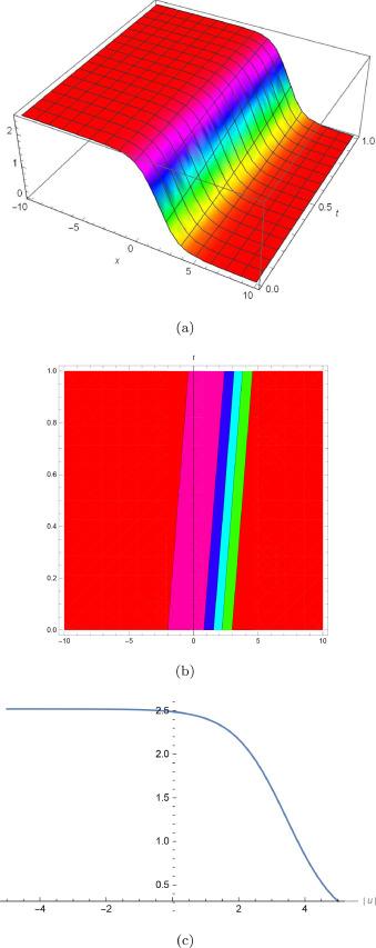
Fig.3 (a) is 3D plot, (b) is contour plot and (c) is 2D plot for solution of $u_{3} (x, t)$ for the values of $d = 3, λ = 0.3, v = - 2, ω = - 5$ and $μ = 0.4$ .

View original graphic|Download|PPT slide

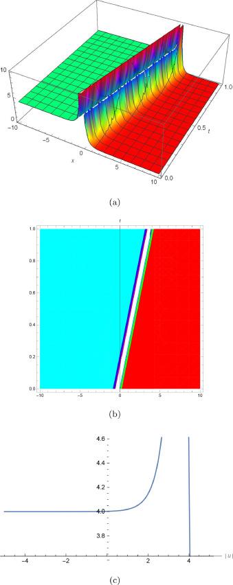
Fig.4 (a) is 3D plot, (b) is contour plot and (c) is 2D plot for solution of $u_{4} (x, t)$ for the values of $d = 3, λ = 2, μ = - 3, ω = - 5$ and $v = 4$ .

View original graphic|Download|PPT slide

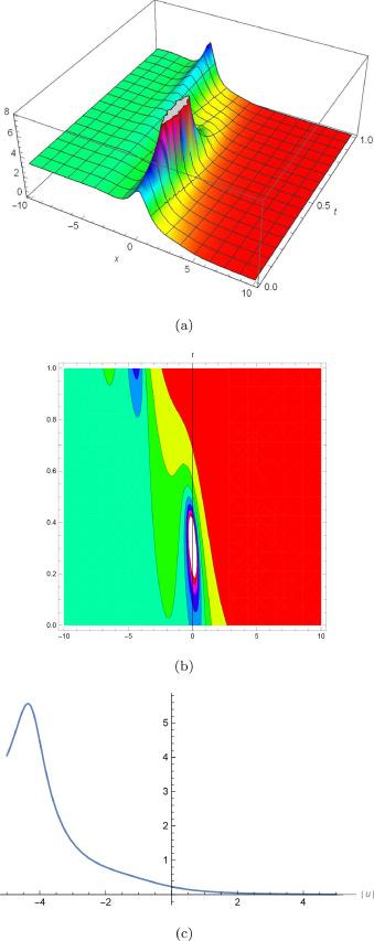
Fig.5 (a) is 3D plot, (b) is contour plot and (c) is 2D plot for solution of $u_{5} (x, t)$ for the values of $d = - 2, λ = 0.5, μ = - 3, ω = 0.3$ and $v = - 4$ .

View original graphic|Download|PPT slide

Fig.6 (a) is 3D plot, (b) is contour plot and (c) is 2D plot for solution of $u_{6} (x, t)$ for the values of $κ = - 4, λ = - 0.5, μ = - 3, ω = - 3$ and $d = - 2$ .

To express the solutions obtained by the

(\frac{1}{G^{'}})

-expansion method, Fig. 7 illustrates

u_{7} (x, y, z, t)

in Case I for

A = 0.3, κ = - 3, λ = 0.4

and

μ = 0.7

; Fig. 8 expresses

u_{8} (x, y, z, t)

established in Case I for

A = 3, λ = - 0.4, v = - 6

and

μ = 7

; Fig. 9 demonstrates

u_{9} (x, y, z, t)

found in Case II for

A = 3, λ = - 0.4, μ = 7

and

v = - 6 .

; while Fig. 10 demonstrates

u_{10} (x, y, z, t)

found in Case III for

A = - 3, λ = - 0.4, μ = 0.7

and

v = 0.2 .

; Fig. 11 represents

u_{11} (x, t)

found in Case I for

A = 3, κ = 0.4, μ = - 4

and

v = 0.6

and Fig. 12 determines

u_{12} (x, t)

found in Case II for

A = - 3, κ = - 0.4, μ = 0.3

and

v = 0.2

View original graphic|Download|PPT slide

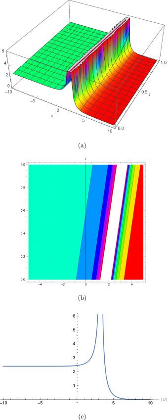
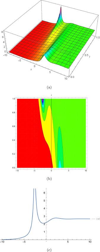
Fig.7 (a) is 3D plot, (b) is contour plot and (c) is 2D plot for solution of $u_{7} (x, t)$ for the values of $A = 0.3, κ = - 3, λ = 0.4$ and $μ = 0.7$ .

View original graphic|Download|PPT slide

Fig.8 (a) is 3D plot, (b) is contour plot and (c) is 2D plot for solution of $u_{8} (x, t)$ for the values of $A = 3, λ = - 0.4, v = - 6$ and $μ = 7$ .

View original graphic|Download|PPT slide

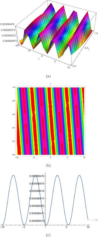
Fig.9 (a) is 3D plot, (b) is contour plot and (c) is 2D plot for solution of $u_{9} (x, t)$ for the values of $A = 3, λ = - 0.4, μ = 7$ and $v = - 6 .$ .

View original graphic|Download|PPT slide

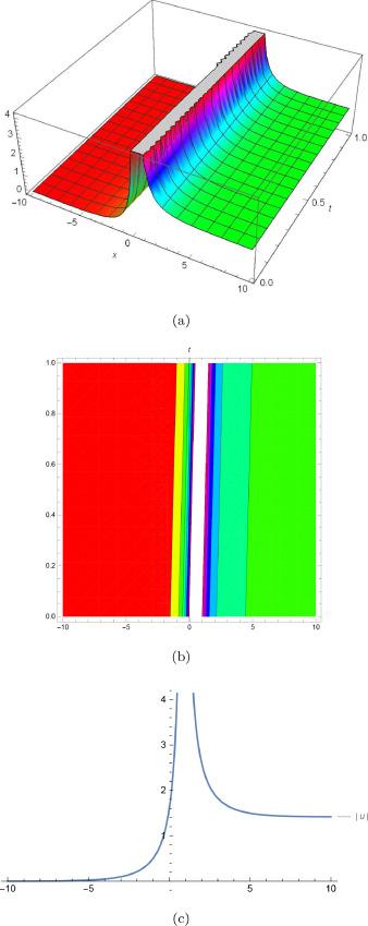
Fig.10 (a) is 3D plot, (b) is contour plot and (c) is 2D plot for solution of $u_{10} (x, t)$ for the values of $A = - 3, λ = - 0.4, μ = 0.7$ and $v = 0.2$ .

View original graphic|Download|PPT slide

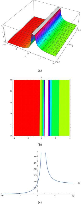
Fig.11 (a) is 3D plot, (b) is contour plot and (c) is 2D plot for solution of $u_{11} (x, t)$ for the values of $A = 3, κ = 0.4, μ = - 4$ and $v = 0.6$ .

View original graphic|Download|PPT slide

Fig.12 (a) is 3D plot, (b) is contour plot and (c) is 2D plot for solution of $u_{12} (x, t)$ for the values of $A = - 3, κ = - 0.4, μ = 0.3$ and $v = 0.2$ .

To demonstrate the solutions developed by the modified Kudrayshov method; Fig. 13 illustrates

u_{13} (x, y, z, t)

established in Case I for

v = - 0.3, a = 3, d = - 6, λ = 0.2

and

μ = - 0.9

while Fig. 14 demonstrates

u_{14} (x, y, z, t)

found in Case II for

a = 2, d = 3, λ = 0.3, μ = - 6

and

v = 8 .

; Fig. 15 demonstrates

u_{15} (x, y, z, t)

found in Case III for

a = 3, d = - 4, λ = 0.3, μ = - 3

and

v = 0.8 .

; Fig. 16 illustrates

u_{16} (x, y, z, t)

established in Case I for

d = 3, κ = 2, λ = 0.3, μ = 3

and

v = 0.8

; Fig. 17 illustrates

u_{17} (x, y, z, t)

established in Case II for

d = 2, κ = 5, λ = 0.3, μ = 8

and

v = 0.8

and Fig. 18 shows

u_{18} (x, y, z, t)

observed in Case I for

a = 0.8, κ = - 4, λ = 0.3, μ = 6

and

d = 3

View original graphic|Download|PPT slide

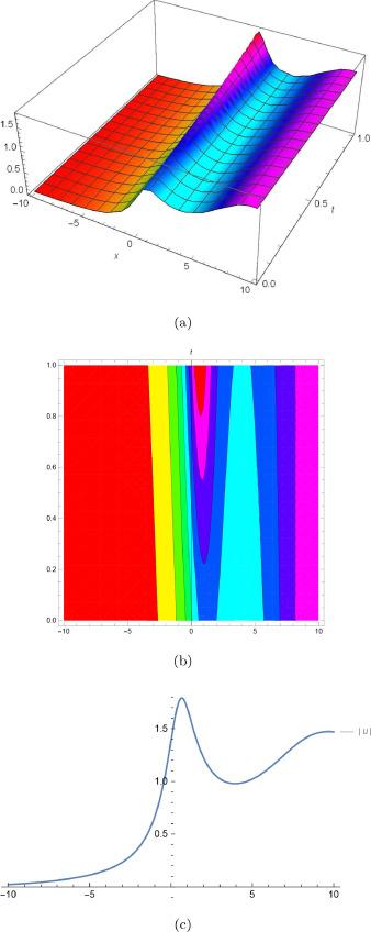
Fig.13 (a) is 3D plot, (b) is contour plot and (c) is 2D plot for solution of $u_{13} (x, t)$ for the values of $v = - 0.3, a = 3, d = - 6, λ = 0.2$ and $μ = - 0.9$ .

View original graphic|Download|PPT slide

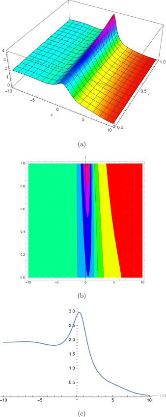
Fig.14 (a) is 3D plot, (b) is contour plot and (c) is 2D plot for solution of $u_{14} (x, t)$ for the values of $a = 2, d = 3, λ = 0.3, μ = - 6$ and $v = 8$ .

View original graphic|Download|PPT slide

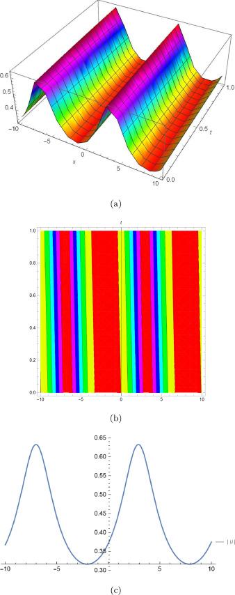
Fig.15 (a) is 3D plot, (b) is contour plot and (c) is 2D plot for solution of $u_{15} (x, t)$ for the values of $a = 3, d = - 4, λ = 0.3, μ = - 3$ and $v = 0.8$ .

View original graphic|Download|PPT slide

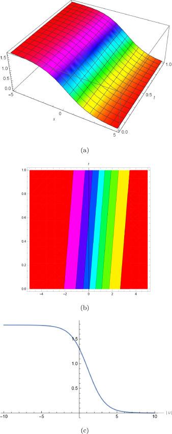
Fig.16 (a) is 3D plot, (b) is contour plot and (c) is 2D plot for solution of $u_{16} (x, t)$ for the values of $d = 3, κ = 2, λ = 0.3, μ = 3$ and $v = 0.8$ .

View original graphic|Download|PPT slide

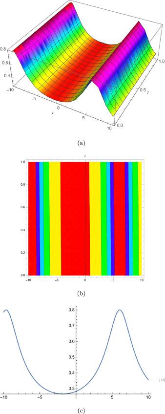
Fig.17 (a) is 3D plot, (b) is contour plot and (c) is 2D plot for solution of $u_{17} (x, t)$ for the values of $d = 2, κ = 5, λ = 0.3, μ = 8$ and $v = 0.8$ .

View original graphic|Download|PPT slide

Fig.18 (a) is 3D plot, (b) is contour plot and (c) is 2D plot for solution of $u_{18} (x, t)$ for the values of $a = 0.8, κ = - 4, λ = 0.3, μ = 6$ and $d = 3$ .

5. Conclusion

In work, some new exact solutions to the generalized (3 + 1)-dimensional Boiti-Leon-Manna-Pempinelli model have been investigated by employing the

(\frac{1}{G^{'}})

-expansion approach, the Bernoulli sub-ODE approach and the modified Kudryashov method. A variety of solitons are observed namely, bright, dark, singular, combo, optical, singular optical, trigonometric functions, trigonometric and hyperbolic functions, and rational solutions and bright-singular combo soliton solutions are demonstrated for details see Fig. 1, Fig. 2, Fig. 3, Fig. 4, Fig. 5, Fig. 6, Fig. 7, Fig. 8, Fig. 9, Fig. 10, Fig. 11, Fig. 12, Fig. 13, Fig. 14, Fig. 15, Fig. 16, Fig. 17, Fig. 18. The computational results are encouraging and can be extended for obtaining novel exact solutions to many complex nonlinear problems arising in engineering and mathematical physics. The symbolic computational work supports the efficacy, reliability, and simplicity of present methodologies. Many higher dimensional nonlinear evolution models that occur in science, mathematical physics, and marine engineering can benefit from these strategies.

Declaration of Competing Interest

The authors declare that they have no known competing financial interests or personal relationships that could have appeared to influence the work reported in this paper.

References

Publishing order | Descend order by publishing year | Descend order by cited within

[1]	M.S. Osman, J. Machado, D. Baleanu. Opt. Quantum Electron., 50 (2) (2018), pp. 1-11

[2]	K.K. Ali, M.S. Osman, M. Abdel-Aty. Alex. Eng. J., 59 (3) (2020), pp. 1191-1196

[3]	S. Kumar, R. Kumar, M.S. Osman, B. Samet. Numer. Methods Partial Differ. Equ.,37 (2) (2021), pp. 1250-1268 DOI: 10.1002/num.22577

[4]	H. Berrehal, F. Mabood, O.D. Makinde. Eur. Phys. J. Plus, 135 (7) (2020), pp. 1-21

[5]	K.K. Ali, A.-M. Wazwaz, M.S. Osman. Optik, 208 (2020), p. 164132

[6]	B. Inan, M.S. Osman, T. Ak, D. Baleanu. Math. Methods Appl. Sci., 43 (5) (2020), pp. 2588-2600 DOI: 10.1002/mma.6067

[7]	Y. Zhang, D. Wang. Fractal Fractional, 5 (2) (2021), p. 39

[8]	K.K. Ali, R. Yilmazer, M.S. Osman. Phys. Scr., 96 (12) (2021), p. 125249 DOI: 10.1088/1402-4896/ac35c5

[9]	M.S. Osman. Pramana, 88 (4) (2017), pp. 1-9 DOI: 10.5958/2231-6701.2017.00016.1

[10]	S. Liu, Z. Fu, S. Liu, Q. Zhao. Phys. Lett. A, 289 (1-2) (2001), pp. 69-74

[11]	M.R. Ali, W.-X. Ma, R. Sadat. J. Ocean Eng. Sci. (2021)

[12]	W.-X. Ma, T. Huang, Y. Zhang. Phys. Scr.,82 (6) (2010), p. 065003 DOI: 10.1088/0031-8949/82/06/065003

[13]	M.A. Abdou. Chaos Solitons Fractals, 31 (1) (2007), pp. 95-104

[14]	H. Triki, A.-M. Wazwaz. Appl. Math. Comput., 214 (2) (2009), pp. 370-373

[15]	S.-Q. Wang, J.-H. He. Chaos Solitons Fractals, 35 (4) (2008), pp. 688-691

[16]	M. Wadati, K. Konno, Y.-H. Ichikawa. A Generalization of Inverse Scattering Method. Technical Report, Nagoya Univ. (Japan). Inst. of Plasma Physics (1979)

[17]	J.-H. He. Int. J. Non Linear Mech., 34 (4) (1999), pp. 699-708

[18]	A.-M. Wazwaz. Appl. Math. Comput., 154 (3) (2004), pp. 713-723

[19]	T.A. Sulaiman, H. Bulut. J. Ocean Eng. Sci., 4 (1) (2019), pp. 1-6

[20]	Z. LÃ¼, H. Zhang. Phys. Lett. A, 324 (4) (2004), pp. 293-298

[21]	E. Fan, H. Zhang. Phys. Lett. A, 246 (5) (1998), pp. 403-406

[22]	M.M.A. Khater, S. Muhammad, A. Al-Ghamdi, M. Higazy. J. Ocean Eng. Sci. (2022)

[23]	J.-H. He. Appl. Math. Comput., 156 (3) (2004), pp. 591-596

[24]	H. Rezazadeh, A.R. Seadawy, M. Eslami, M. Mirzazadeh. J. Ocean Eng. Sci., 4 (2) (2019), pp. 77-84

[25]	A.-M. Wazwaz. J. Ocean Eng. Sci., 1 (3) (2016), pp. 181-185

[26]	M.S. Osman, H. Almusawa, K.U. Tariq, S. Anwar, S. Kumar, M. Younis, W.-X. Ma. J. Ocean Eng. Sci. (2021)

[27]	F. Rahimi, T. Ghaffary, Y. Naimi, H. Khajehazad. Opt. Quantum Electron., 53 (1) (2021), pp. 1-16 DOI: 10.1504/ijma.2021.10036210

[28]	A. Biswas, Y. Yildirim, E. Yasar, Q. Zhou, S.P. Moshokoa, M. Belic. Optik, 160 (2018), pp. 24-32

[29]	Y.S. Ã-zkan, E. YaÅŸar, A.R. Seadawy. J. Taibah Univ. Sci., 14 (1) (2020), pp. 585-597 DOI: 10.1080/16583655.2020.1760513

[30]	M. Mirzazadeh, Y. YÄ±ldÄ±rÄ±m, E. YaÅŸar, H. Triki, Q. Zhou, S.P. Moshokoa, M.Z. Ullah, A.R. Seadawy, A. Biswas, M. Belic. Optik, 154 (2018), pp. 551-557

[31]	E. YaÅŸar. Appl. Math. Comput., 216 (11) (2010), pp. 3191-3194

[32]	E. YaÅŸar, Y. YÄ±ldÄ±rÄ±m, E. YaÅŸar. Results Phys., 9 (2018), pp. 1666-1672

[33]	E. YaÅŸar, S. San, Y.S. Ã-zkan. Open Phys.,14 (1) (2016), pp. 37-43 DOI: 10.1515/phys-2016-0007

[34]	N.A. Kudryashov. Commun. Nonlinear Sci. Numer. Simul., 17 (6) (2012), pp. 2248-2253

[35]	M.S. Osman. Open Phys.,14 (1) (2016), pp. 26-36 DOI: 10.1515/phys-2015-0056

[36]	H.I. Abdel-Gawad, M. Osman. Indian J. Pure Appl. Math., 45 (1) (2014), pp. 1-12 DOI: 10.1007/s13226-014-0047-x

[37]	K. Hosseini, M. Matinfar, M. Mirzazadeh. Regul. Chaotic Dyn., 26 (1) (2021), pp. 105-112 DOI: 10.1134/s1560354721010068

[38]	M. Darvishi, M. Najafi, L. Kavitha, M. Venkatesh. Commun. Theor. Phys.,58 (6) (2012), p. 785 DOI: 10.1088/0253-6102/58/6/01

[39]	X.-Y. Gao. Zeitschrift fÃ¼r Naturforschung A, 70 (1) (2015), pp. 59-61 DOI: 10.1515/zna-2014-0272

[40]	B.-Q. Li, Y.-L. Ma. Comput. Math. Appl., 76 (1) (2018), pp. 204-214

[41]	A.-M. Wazwaz. Int. J. Numer. Methods Heat Fluid Flow (2020)

[42]	M.S. Osman, A.-M. Wazwaz. Math. Methods Appl. Sci., 42 (18) (2019), pp. 6277-6283 DOI: 10.1002/mma.5721

[43]	M.R. Ali, W.-X. Ma. Adv. Math. Phys., 2019 (2019)

Options

Outlines

模态框（Modal）标题

Abstract

Cite this article

1. Introduction

2. Methodology

2.1. The Bernoulli sub-ode method

2.2. The (1G′) -expansion method

2.3. The modified Kudryashov method

3. Mathematical analysis

3.1. Applications to the Bernouli sub-ode method

3.2. Applications of (1G′) -expansion method

3.3. Applications to the modified Kudrayshov method

4. Discussion and results

Fig.1 (a) is 3D plot, (b) is contour plot and (c) is 2D plot for solution of u1(x,t) for the values of d=3,κ=2,μ=8,v=4 and ω=6 .

Fig.2 (a) is 3D plot, (b) is contour plot and (c) is 2D plot for solution of u2(x,y,t) for the values of d=−7,κ=−8,μ=3,ω=5 and v=2 .

Fig.3 (a) is 3D plot, (b) is contour plot and (c) is 2D plot for solution of u3(x,t) for the values of d=3,λ=0.3,v=−2,ω=−5 and μ=0.4 .

Fig.4 (a) is 3D plot, (b) is contour plot and (c) is 2D plot for solution of u4(x,t) for the values of d=3,λ=2,μ=−3,ω=−5 and v=4 .

Fig.5 (a) is 3D plot, (b) is contour plot and (c) is 2D plot for solution of u5(x,t) for the values of d=−2,λ=0.5,μ=−3,ω=0.3 and v=−4 .

Fig.6 (a) is 3D plot, (b) is contour plot and (c) is 2D plot for solution of u6(x,t) for the values of κ=−4,λ=−0.5,μ=−3,ω=−3 and d=−2 .

Fig.7 (a) is 3D plot, (b) is contour plot and (c) is 2D plot for solution of u7(x,t) for the values of A=0.3,κ=−3,λ=0.4 and μ=0.7 .

Fig.8 (a) is 3D plot, (b) is contour plot and (c) is 2D plot for solution of u8(x,t) for the values of A=3,λ=−0.4,v=−6 and μ=7 .

Fig.9 (a) is 3D plot, (b) is contour plot and (c) is 2D plot for solution of u9(x,t) for the values of A=3,λ=−0.4,μ=7 and v=−6. .

Fig.10 (a) is 3D plot, (b) is contour plot and (c) is 2D plot for solution of u10(x,t) for the values of A=−3,λ=−0.4,μ=0.7 and v=0.2 .

Fig.11 (a) is 3D plot, (b) is contour plot and (c) is 2D plot for solution of u11(x,t) for the values of A=3,κ=0.4,μ=−4 and v=0.6 .

Fig.12 (a) is 3D plot, (b) is contour plot and (c) is 2D plot for solution of u12(x,t) for the values of A=−3,κ=−0.4,μ=0.3 and v=0.2 .

Fig.13 (a) is 3D plot, (b) is contour plot and (c) is 2D plot for solution of u13(x,t) for the values of v=−0.3,a=3,d=−6,λ=0.2 and μ=−0.9 .

Fig.14 (a) is 3D plot, (b) is contour plot and (c) is 2D plot for solution of u14(x,t) for the values of a=2,d=3,λ=0.3,μ=−6 and v=8 .

Fig.15 (a) is 3D plot, (b) is contour plot and (c) is 2D plot for solution of u15(x,t) for the values of a=3,d=−4,λ=0.3,μ=−3 and v=0.8 .

Fig.16 (a) is 3D plot, (b) is contour plot and (c) is 2D plot for solution of u16(x,t) for the values of d=3,κ=2,λ=0.3,μ=3 and v=0.8 .

Fig.17 (a) is 3D plot, (b) is contour plot and (c) is 2D plot for solution of u17(x,t) for the values of d=2,κ=5,λ=0.3,μ=8 and v=0.8 .

Fig.18 (a) is 3D plot, (b) is contour plot and (c) is 2D plot for solution of u18(x,t) for the values of a=0.8,κ=−4,λ=0.3,μ=6 and d=3 .

5. Conclusion

Declaration of Competing Interest

References

Links

2.2. The $(\frac{1}{G^{'}})$ -expansion method

3.2. Applications of $(\frac{1}{G^{'}})$ -expansion method

Fig.1 (a) is 3D plot, (b) is contour plot and (c) is 2D plot for solution of $u_{1} (x, t)$ for the values of $d = 3, κ = 2, μ = 8, v = 4$ and $ω = 6$ .

Fig.2 (a) is 3D plot, (b) is contour plot and (c) is 2D plot for solution of $u_{2} (x, y, t)$ for the values of $d = - 7, κ = - 8, μ = 3, ω = 5$ and $v = 2$ .

Fig.3 (a) is 3D plot, (b) is contour plot and (c) is 2D plot for solution of $u_{3} (x, t)$ for the values of $d = 3, λ = 0.3, v = - 2, ω = - 5$ and $μ = 0.4$ .

Fig.4 (a) is 3D plot, (b) is contour plot and (c) is 2D plot for solution of $u_{4} (x, t)$ for the values of $d = 3, λ = 2, μ = - 3, ω = - 5$ and $v = 4$ .

Fig.5 (a) is 3D plot, (b) is contour plot and (c) is 2D plot for solution of $u_{5} (x, t)$ for the values of $d = - 2, λ = 0.5, μ = - 3, ω = 0.3$ and $v = - 4$ .

Fig.6 (a) is 3D plot, (b) is contour plot and (c) is 2D plot for solution of $u_{6} (x, t)$ for the values of $κ = - 4, λ = - 0.5, μ = - 3, ω = - 3$ and $d = - 2$ .

Fig.7 (a) is 3D plot, (b) is contour plot and (c) is 2D plot for solution of $u_{7} (x, t)$ for the values of $A = 0.3, κ = - 3, λ = 0.4$ and $μ = 0.7$ .

Fig.8 (a) is 3D plot, (b) is contour plot and (c) is 2D plot for solution of $u_{8} (x, t)$ for the values of $A = 3, λ = - 0.4, v = - 6$ and $μ = 7$ .

Fig.9 (a) is 3D plot, (b) is contour plot and (c) is 2D plot for solution of $u_{9} (x, t)$ for the values of $A = 3, λ = - 0.4, μ = 7$ and $v = - 6 .$ .

Fig.10 (a) is 3D plot, (b) is contour plot and (c) is 2D plot for solution of $u_{10} (x, t)$ for the values of $A = - 3, λ = - 0.4, μ = 0.7$ and $v = 0.2$ .

Fig.11 (a) is 3D plot, (b) is contour plot and (c) is 2D plot for solution of $u_{11} (x, t)$ for the values of $A = 3, κ = 0.4, μ = - 4$ and $v = 0.6$ .

Fig.12 (a) is 3D plot, (b) is contour plot and (c) is 2D plot for solution of $u_{12} (x, t)$ for the values of $A = - 3, κ = - 0.4, μ = 0.3$ and $v = 0.2$ .

Fig.13 (a) is 3D plot, (b) is contour plot and (c) is 2D plot for solution of $u_{13} (x, t)$ for the values of $v = - 0.3, a = 3, d = - 6, λ = 0.2$ and $μ = - 0.9$ .

Fig.14 (a) is 3D plot, (b) is contour plot and (c) is 2D plot for solution of $u_{14} (x, t)$ for the values of $a = 2, d = 3, λ = 0.3, μ = - 6$ and $v = 8$ .

Fig.15 (a) is 3D plot, (b) is contour plot and (c) is 2D plot for solution of $u_{15} (x, t)$ for the values of $a = 3, d = - 4, λ = 0.3, μ = - 3$ and $v = 0.8$ .

Fig.16 (a) is 3D plot, (b) is contour plot and (c) is 2D plot for solution of $u_{16} (x, t)$ for the values of $d = 3, κ = 2, λ = 0.3, μ = 3$ and $v = 0.8$ .

Fig.17 (a) is 3D plot, (b) is contour plot and (c) is 2D plot for solution of $u_{17} (x, t)$ for the values of $d = 2, κ = 5, λ = 0.3, μ = 8$ and $v = 0.8$ .

Fig.18 (a) is 3D plot, (b) is contour plot and (c) is 2D plot for solution of $u_{18} (x, t)$ for the values of $a = 0.8, κ = - 4, λ = 0.3, μ = 6$ and $d = 3$ .