
1 Introduction
Terrestrial ecosystem stores a large quantity of carbon (C) in plant and soil [1,2,3,4], and constitutes an important C sink of the Earth, with annual net C uptake of 2.0-3.4 Pg C per year (1 Pg = 1015 g) [5,6,7]. The Intergovernmental Panel on Climate Change (IPCC) estimated that the global soil annual C sequestration ranged from 0.6 to 1.2 Pg C, and China was one of the highest soil C sequestration countries in the world [8,9,10]. Specially, the Chinese land biosphere sink was 11 Pg (1015 g) of C during 2010 to 2016, and in the next 40 years (2021-2060), the potential C sink of Chinese land biosphere is about 3.0-3.6 Pg of C [11,12,13,14,15]. A new paper reported that terrestrial C sink of 0.20-0.25 Pg C yr− 1 in China during the past decades, and predicted it to be 0.15-0.52 Pg C yr− 1 by 2060 [15], and the total terrestrial ecosystem C pool in China was about 89 Pg C (vegetation, 14 Pg; soil (0-1 m), 75 Pg) [6].
Over recently decades, vegetation restoration project has been extensively adopted in many countries and regions for economic, ecological and climate change mitigation purposes [16,17,18,19,20,21,22,23,24]. Vegetation restoration reduces soil erosion and CO2 release to the atmosphere, which further increases soil C sequestration [25,26,27]. The ecosystem C stocks increased due to China’s national ecological restoration project [28,29,30,31]. Specially, the Chinese Loess Plateau is one of the most typical regions for vegetation restoration [32,33,34,35]. With increasing scientific and political interest in regional aspects of the global C cycle, there is a strong impetus to better understand the ecosystem C stock of the Loess Plateau [32,33]. In fact, soil C sequestration, distribution and stocks depending on land use types or vegetation restoration of the Loess Plateau has been largely described [36,37]. Though most of works have been conducted on C pools in various ecosystems, there are huge discrepancies in these estimations [32,36,38,39]. Such inconsistency can be ascribed to the limited samples, multiplicity of data sources, and difference in methodologies. For example, previous estimates at both regional and national scales were primarily obtained based on summarized data of the references and not from original studies [6,29]. Therefore, our knowledge of the driving forces causing the changes in ecosystem C stocks on the Loess Plateau is also very limited.
Improving estimate of the size and spatial distribution of C stocks of the Loess Plateau is urgently needed for global C balance. Here, we made the wall-to-wall estimation of C stock in various pools of the Loess Plateau. The C stocks are estimated for plants and soils, including above-ground, below-ground, soil organic C (0-20 cm) stocks for entire the Loess Plateau. We grouped all sites to forestland, shrubland, grassland, and farmland, which can represent the main ecosystem types in this region. Climate data (temperature, precipitation) and soil properties were gathered across the whole Loess Plateau. The following hypothesis was tested: there was a critical role of climate factors in shaping the distribution of ecosystem C density. In this case, the following objectives were to assess the whole ecosystem C stocks across the Loess Plateau, and to investigate how climate factors affect ecosystem C stocks on a large scale. Thus, we employed a geostatistical semivariance fitting to acquire the large-scale ecosystem C stocks. To address the second objective, we applied structural equation models and variation partitioning analysis to explore the impacts of climate factors and soil properties on ecosystem C stocks.
2 Materials and methods
2.1 Study area
The Loess Plateau (100°52′-114°33′E, 33°41′-41°16′N) is within the semi-humid to semi-arid area in northwest China, which covers altogether 64 × 104 km2, 6.5% of the overall area of China. This area is mountain-surrounded, with high complexity of topographic structures, which include basins, sub-plateaus, gullies and hills, and its elevation is 200-3000 m a.s.l. The temperate, semi-arid and arid continental monsoon climate is predominant. The annual average temperature is within the range from 3.6 °C to 14.3 °C, and annual precipitation ranges from 150 mm to 800 mm, mostly concentrated in June and September (55-78%). The parent materials for the soils are yellow loess or wind deposited materials that results in widespread soils with clay loamy texture. Silt-loamy soils take up around 90% of the Loess Plateau, with silt level being 60-75% in most soils [40]. The vegetation alters between forest from forest steppe, typical steppes and semidesert steppes from southeast to northwest.
2.2 Sampling set
In line with arid and semiarid region classification standards, we classified all sampling sites (as well as related datasets) as 3 groups based on annual precipitation including < 250, 500-250 as well as > 500 mm. We further classified annual temperature datasets as 3 groups including < 5, 5-10, together with > 10 °C. Ecosystem types were divided according to land use to four groups: farmland, grassland, shrubland and forestland. The land cover/use data was the annual dataset of land cover in China from 1985 to 2019 [41].
To obtain the latest ecosystem C data, we analyzed 97 × 3 sampling sites across the Loess Plateau (Fig. 1) between July and October, 2021. In each site, we set three duplicate plots (100 m × 100 m) to vegetation survey and soil sampling. All sampling sites were localized by a GPS receiver (horizontal precision, 5 m) and grouped later to representing major ecosystem type, vegetation and topography types (Table S1).
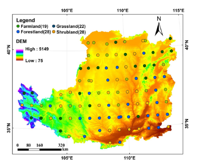
Fig. 1 Distribution of sampling sites in four ecosystem types (Farmland, 19; Grassland, 22; Forestland, 28; Shrubland, 28) across the Loess Plateau. Digital elevation models (DEMs) represent the elevation across the Loess Plateau. DEM data were downloaded from the United States Geological Survey and are free for public use. The figure was generated with ArcGIS 10.0 (http://www.esri.com/) |
Soil was sampled using the auger (diameter, 5 cm), and collected samples at intervals of 10 cm: 0-10 cm and 10-20 cm soil layers from 5 locations of every plot in the radius of 10 m. In every layer, we merged those 5 samples manually for forming the typical sample of respective layer at that site. We harvested undisturbed soil in 0-10 cm as well as 10-20 cm soil layers, and sealed them within the leak tight containers to measure bulk density.
2.3 Estimation of plant C stocks
As for forestland, three standard 20 m × 20 m plots were randomly established within each forestland according to on-site inspection. Species names, diameter at breast height (DBH) and height (H) were documented for all trees within each plot. Specially, we surveyed all trees > 5 cm DBH and height in each of plot, and three standard trees were chosen and logged from standard sampling plots for biomass determination, using the segmenting method. Standard trees were divided into four components: trunk, stem, branches and leaves. Above-ground biomass (AGB) was calculated by summing the trunk, stem, branches and leaves mass of individual trees, using the following component-wise allometric equations (Table 1). Then the above-ground and below-ground biomass were added to derive total biomass.
Table 1 Biomass models and parameters of different trees. Note: WS meas biomass of trunk; WP meas biomass of stem; WB meas biomass of branches; WL meas biomass of leaves; WT meas total above-ground biomass; WR meas total below-ground biomass |
| Tree species | Biomass models and parameters |
|---|---|
| Picea asperata | WT = 0.067732(D2H)0.865949; WR = 0.0088D2.53827 |
| Hemlock | WT = 0.149707(D2H)0.80139; WR = 0.19758D0.6058 |
| Larix gmelini | WT = 0.046238(D2H)0.905002; WR = WT/4.81 |
| Pinus tabuliformis | WS = 0.027636(D2H)0.9905; WB = 0.0091313(D2H)0.982 WL = 0.0045755(D2H)0.9894; WT = WS+ WB+ WL; WR = 0.0084800D0.988 |
| Pinus armandi | WS = 0.01308(D2H)1.0038; WB = 0.0055(D2H)1.0439 WL = 0.0011(D2H)1.12566; WT = WS+ WB+ WL; WR = 0.0033D1.0148 |
| Pinus massoniana | WT = 0.071556(D2H)0.857209; WR = WT/6.23 |
| Cunninghamia | WS = 0.073429(D2H)0.86262; WP = 0.013775(D2H)0.84463; WB = 0.000482(D2H)1.23314 WL = 0.019638(D2H)0.78969; WT = WS+ WP |
| Cupressus | WS = 0.12531(D2H)0.733; WB = 0.137403 + 0.012887D2H WL = 0.05349 + 0.00997D2H; WT = WS+ WB+ WL; WR = 0.01109 D2H-0.160386 |
| Betula | WT = 0.0278601(D2H)0.993386; WR = WT/2.89 |
| Broad-leaved forest | WS = 0.044(D2H)0.9169; WP = 0.023(D2H)0.7115; WB = 0.0104(D2H)0.9994; WL = 0.0188(D2H)0.8024; WT = WS+ WP+ WB+ WL; WR = 0.0197D0.8963 |
| Coniferous forest | WT = 0.0495502(D2H)0.952453; WR = WT/3.85 |
For below-ground biomass (BGB), as the excavation of entire trees is very time- and labor-consuming and destructive, we only dig the root in 0-20 cm by the skeleton method (dry excavation), and fresh weights of these components were determined in the field. The component parts were later sub-sampled for moisture determination and C concentration analysis. Each subsample was taken to the laboratory and oven-dried at 60 °C to a constant weight. Dry weights of every component were determined and mechanically ground into pass through a 0.5 mm mesh screen. In addition, air-dried soil samples were treated with 10% hydrochloric acid for 12 h to remove carbonates, dried at 70 °C for 48 h, milled, and passed through a 0.25 mm mesh screen. The powder samples of different components were analyzed for the C concentrations using a vario macro elemental analyzer (Elementar Analysensysteme GmbH, Germany). The carbon storage in the tree components is estimated as follows [42]:
$\mathrm{Carbon}\;\mathrm{storage}\;\mathrm{in}\;\mathrm{each}\;\mathrm{stand}\:=\:(\mathrm{carbon}\;\mathrm{content}\;\mathrm{in}\;\mathrm{different}\;\mathrm{components}\;\times\;\mathrm{biomass}\;\mathrm{in}\;\mathrm{different}\;\mathrm{components}$
As for shrubland, grassland and cropland, the above-ground biomass (AGB) as well as below-ground biomass (BGB) was collected in the 5 plots (1 × 1 m). The roots were excavated as completely as possible in 0-20 cm soil depth, and separated into fine roots (< 2 mm diameter) and coarse roots (> 2 mm diameter). Both the coarse and fine roots were weighed in the field. The portion of the stump that remains underground was treated as a part of the coarse root. The root samples in triplicate were brought to the laboratory and oven-dried at 80 °C till constant weight was achieved [43]. Also, carbon storage in each stand = (carbon content in different components × biomass in different components.
Apart from that, we collected dead above-ground biomass samples but did not consider them for eventual measurements. According to our results, dead biomass for just 0.1% of overall biomass for forestland and shrubland, and it had almost no effect on C stocks.
2.4 Estimation of soil C stocks
We sieved soil samples through the 2.0-mm mesh to exclude some gravel and plant residual roots [44], to determine soil texture (%) by laser diffraction using a Mastersizer 2000 (Malvern Instruments, England). The soil bulk density (g cm− 3) was determined in the original undisturbed soil core dry mass volume following oven-drying under 105 °C.
The total soil C density (SOCD, kg·m− 2) was quantitatively measured by collecting soil at 0-20 cm depth. SOCD was computed as [16]:
$\textrm{SOCD}=\textrm{SOC}\times \textrm{BD}\times \textrm{D}/10$
SOC refers to soil organic carbon (g·kg− 1), BD indicates soil bulk density (g·cm− 3) and D suggests soil thickness (cm).
$\textrm{ETCD}=\textrm{AGCD}+\textrm{BGCD}+\textrm{SOCD}$
AGCD means above-ground C density, BGCD means below-ground C density, ETCD means the ecosystem total C density.
2.5 Estimation of ecosystem C stocks
To estimate ecosystem C stocks, data on the AGCD, BGCD, SOCD, ETCD as well as the area of the research region are needed. With optimal interpolation, Geostatistics is applied to convert AGCD, BGCD, SOCD and ETCD dataset from discrete points to a spatially continuous surface. With the application of regionalized variable theory [45], geostatistics adopts semivariograms [46] for quantifying spatial autocorrelations and afford input parameters to spatial interpolation, including kriging. An empirically derived semivariogram can be written as:
$\gamma (h)=\frac{1}{2N(h)}\sum_{i=1}^{N(h)}{\left[z(xi)-z\left( xi+h\right)\right]}^2$
where N(h) means the sample amount at every distance interval h, and z (xi), z(xi + h) suggests the value obtained through dividing soil moisture of any two samples by lag distance h.
Subsequently, standard theoretical models (such as spherical, Gaussian, exponential and linear models), were fitted to the empirical semivariogram based on measured data. The best fitted model, with minimum residual sum of squares and maximum determination coefficient, was applied to present input parameters to kriging interpolation. The equations applied for the above-mentioned models are presented as:
Linear model:
$\gamma (h)= Co+C\left[\left(h/ Ao\right)\right]$
Spherical model:
$\gamma (h)= Co+C\left[1.5\left(h/ Ao\right)-0.5\left(h/ Ao\right)3\right],h\le Ao$
$\gamma (h)= Co+C,h\ge Ao$
Exponential model:
$\gamma (h)= Co+C\left[1-\left(\mathit{\sin}\left(h/ Ao\right)\times h/ Ao\right)\right]$
where Co indicates the nugget variance, i.e., the y intercept in the model suggesting the measurement error or variance at a shorter distance; C suggests the asymptote of semivariance γ(h); Co + C means the sill and Ao represents the range, as an index for area (auto-correlation) similarity in the tested samples, relying upon both study area and sampling patterns. Spatial dependence, frequently expressed as (C/[(C + Co]), links small-scale variability to large-scale variability.
After the spatial interpolation, AGCD, BGCD and SOCD surface were formed to contain the whole area of the Loess Plateau. The surface was exported as a raster layer having a defined resolution (3000 m × 3000 m), with every grid square assigned with AGCD, BGCD, and SOCD value and an area value. Based on the Spatial Analyst module, AGCs (AGC stock), BGCs (BGC stock) and SOCs (SOC stock) (Pg; 1015 g) were carried out by adopting the GIS software package Arcmap Desktop (version 9.1). Finally, ETCs (ETC stock) was calculated by AGCs + BGCs + SOCs.
According to previous studies, random forest grows a large number of regression trees from different random subsets of training data and predictor variables, thereby reducing variance relative to single trees, and greatly reducing the risk of over-fitting model predictions and non-optimal solutions— though at the cost of interpretability [47]. In this case, we tried to estimate soil C stocks by random forest model compared with the spatial interpolation method (Tables S2 and S3). The predicted results from random forest are similar to those of kriging interpolation. There was the lower p value and the higher R2 in kriging interpolation model, and the standard error of the mean, root mean square error of kriging interpolation were lower. It means that the precision of the model of kriging interpolation was better than random forest model for ecosystem C stocks. This is possible because that there was no more topographic and vegetation data, climate data, and remote-sensing image, therefore, there was error transfer and accumulation when using random forests to extract these environmental explanatory variables, moreover, the complex terrain across the Loess Plateau made the verification results were not satisfactory. Thus, if we made the total ecosystem carbon stocks, the interpolation methods should be consistent. Based on these reasons, kriging interpolation was selected to calculate the ecosystem C stocks and their factors across Loess Plateau.
2.6 Climate factors and soil properties
Mean annual temperature (MAT, °C) and precipitation (MAP, mm) were measured using meteorological data between 1953 and 2013 from China Meteorological Data Sharing Service System (http://cdc.cma.gov.cn/). This dataset covers climatic data of 64 national-level weather stations near or on the Loess Plateau. Later, we interpolated those data in respective stations by kriging to create continuous data surfaces of the meteorological variables. Afterwards, we utilized sampling sites’ spatial coordinates for extracting their meteorological parameters from respective data surface. Soil pH was determined by the soil-water extraction (1:1.5, v/v). We utilized Kjeldahl approach [48] for measuring soil total nitrogen (TN, g·kg− 1). Soil cation exchange capacity (CEC, cmol kg− 1) was determined based on Tucker’s method [49] using a leaching device. Summary of soil properties and their geostatistical parameters in different ecosystems were shown in Tables S4 and S5.
2.7 Data analysis
Kolmogorov-Smirnov test was used to determine whether ecosystem C density followed a normal distribution. All data were checked using SAS v.9.3 (https://www.sas.com/zh_cn/software/platform.html) through one-way ANOVA followed by performing Fisher’s test (p < 0.05). Linear regression analysis was used to explore the relationships among ecosystem C densities. The R software (http://www.datavis.ca/R/) with ‘varpart’ package was used for variation partitioning analysis. Pearson’s correlation coefficients were adopted for determining the relationships between environmental factors and ecosystem C stocks, and then, heatmaps were made by using ‘pheatmap’ package.
Finally, structural equation models (SEMs) were used to explain the effects of climate factors (MAT, MAP) and soil properties (TN, CEC, pH, Clay) on the ecosystem C stocks. The final SEMs were constructed using the Mantel R-values in AMOS v. 21.0 (https://www.ibm.com/). The criteria used to evaluate the suitability of the SEMs included the decreased chi-square value (χ2), the decreased root mean square error of approximation (RMSEA< 0.05), the increased comparative fit index (CFI > 0.90), the decreased Akaike information criterion value (AIC), as well as non-significance (p > 0.05).
3 Results
3.1 Spatial distribution of C densities across the loess plateau
Spatial distribution of SOCD (0-10 and 10-20 cm), AGCD, BGCD and ETCD by geostatistical approaches showed the nugget-to-sill ratios of 0.22 and 2.0 (Table S6). No anisotropy was detected, while the spherical model/ exponential model/ linear model well fitted the isotropic semivariograms (Table S6). The SOC, SOCD and ETCD were presented in spherical model, while AGCD and BGCD were presented in the exponential and linear models, respectively.
Kriging interpolation resulted in the continuous SOC, SOCD, AGCD, BGCD and ETCD, which covered the whole Loess Plateau area. There was a strong linear relation between SOC/SOCD in 0-10 cm and 10-20 cm (p < 0.05) (Fig. S1), but a quadratic equation relation between AGCD and BGCD (p < 0.05) (Fig. S2).
Here, ETCD reduced from southeast to northwest, with uneven distribution within eastern and western Loess Plateau (Fig. 2). The AGCD showed a zonal distribution (Fig. 3), SOCD was higher at the depth of 0-10 cm compared with 10-20 cm, and gradually decreased from southeast to northwest (Fig. 3). However, BGCD showed the inhomogeneous distribution across the Loess Plateau (Fig. 3).
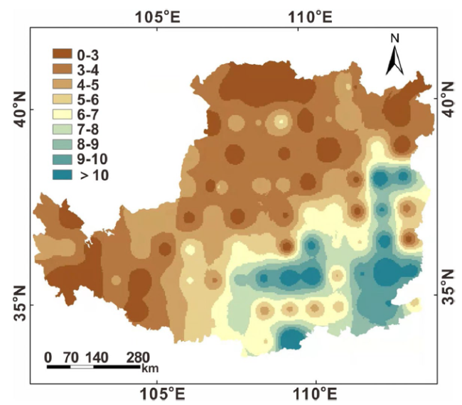
Fig. 2 Spatial pattern of ecosystem total carbon density (ETCD) along longitude and latitude across the Loess Plateau |
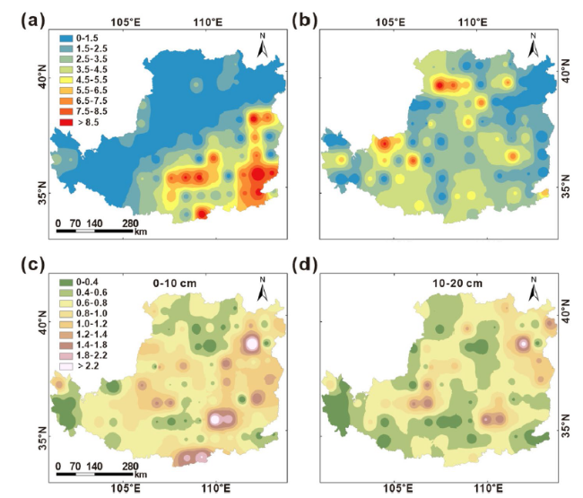
Fig. 3 Spatial distribution of above-ground carbon density (AGCD) (a), below-ground carbon density (BGCD) (b), soil organic carbon density (SOCD) in 0-10 cm layer (c), and soil organic carbon density (SOCD) in 10-20 cm layer (d) across the Loess Plateau |
3.2 Carbon stocks across the loess plateau
The C stocks in ecosystem types across the Loess Plateau (Fig. 4) contain 1.05, 1.18, 0.24 and 0.36 Pg C for farmland, grassland, shrubland and forestland, respectively. The SOC stock in the 0-10 and 10-20 cm soil were 0.47 and 0.37 Pg C, respectively. The above-ground and below-ground C stocks were 1.51 and 0.49 Pg C, respectively.
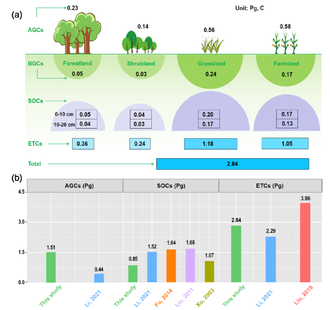
Fig. 4 Summary of the ecosystem C stocks across the Loss Plateau of China (a). Statistics of C density and stocks in the Loess Plateau and China derived from various studies, compared with our study (b). AGCs: above-ground carbon stock; BGCs: below-ground carbon stock; SOCs: soil organic carbon stock; ETCs: ecosystem total carbon stock |
3.3 Carbon densities across ecosystems and climate zones
The SOCD was higher than AGCD and BGCD in farmland and grassland (Fig. 5), while SOCD was lower than AGCD in shrubland and forestland. The SOCD increased according: shrubland < forestland < farmland < grassland. The AGCD and BGCD in forestland and shrubland were higher than farmland and grassland. The SOCD gradually decreased from farmland to forestland, while AGCD increased.
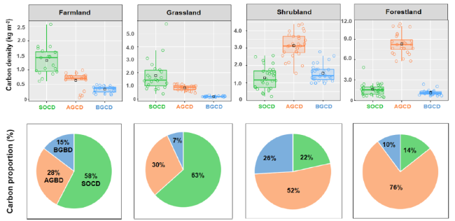
Fig. 5 Box plots show the C density in above-ground, below-ground and soil in farmland, grassland, shrubland, forestland. The lower and upper boundaries of the box represent the first and third quartiles, respectively; the horizontal line represents the mean; the bounds of the lower and upper bars reflect the 10th and 90th percentiles, respectively. The proportion of above-ground carbon density (AGCD), below-ground carbon density (BGCD) and soil organic carbon density (SOCD) in the ecosystem total carbon density (ETCD) in farmland, grassland, shrubland, forestland Average mean annual temperature (MAT) and precipitation (MAP) impacted ecosystem C densities depending on ecosystem types (Fig. S3). The SOCD was obviously higher in zones with temperature higher than 10 °C. The AGCD and BGCD, ETCD in zones with temperature lower than 5 °C were higher than in warmer climate. The SOCD had the same trend as those of AGCD and BGCD. Thus, the ETCD was obviously higher in zones with temperature lower than 5 °C, compared with those with the temperature higher than 10 °C (p < 0.05). Similarly, SOCD, AGCD and ETCD showed the same change trend, and increased within zones with precipitation higher than 500 mm, although BGCD increased within precipitation lower than 250 mm. Thus, wetter and warmer conditions contributed to superior biomass productivity and so, to ecosystem C accumulation. |
3.4 Effects of climate conditions and soil properties on C densities
According to Pearson correlation analysis, ecosystem C densities were strongly dependent on climate factors and soil properties (Fig. 6). The SOCD and ETCD in farmland decreased with mean annual precipitation (MAP), mean annual temperature (MAT) and pH, while increased with soil total nitrogen (TN). The ETCD in grassland, shrubland and forestland increased with MAP while negatively related to MAT. The SOCD in grassland, shrubland and forestland raised with soil clay and TN, while dropped with soil pH (p < 0.05).
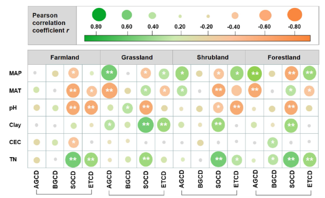
Fig. 6 Pearson correlation between C density and climate factors and soil properties for four ecosystem types. The color of each roundness is proportional to the value of Pearson’s correlation coefficient. Green indicates a positive correlation (dark green, r = 0.80); orange indicates a negative correlation (dark orange, r = 0.80). * p < 0.05; ** p < 0.01. AGCD: above-ground carbon density; BGCD: above-ground carbon density; SOCD: soil organic carbon density; ETCD: ecosystem total carbon density; MAP: mean annual precipitation; MAT: mean annual temperature; pH: soil pH; TN: soil total nitrogen; CEC: soil cation exchange capacity |
Climate factors used in the variation partitioning analysis explained 59%, 56%, 66% and 64% of the total variance of ABGD, BGCD, SOCD and ETCD, while soil properties explained 41%, 44%, 34% and 36% of the total variance of ABGD, BGCD, SOCD and ETCD, respectively (Fig. 7). The most important factors controlling ABGD and BGCD were MAP, TN (p < 0.01). The SOCD were mainly dependent on MAT and TN (p < 0.01), while the ETCD were dependent on MAT and MAP (p < 0.01).
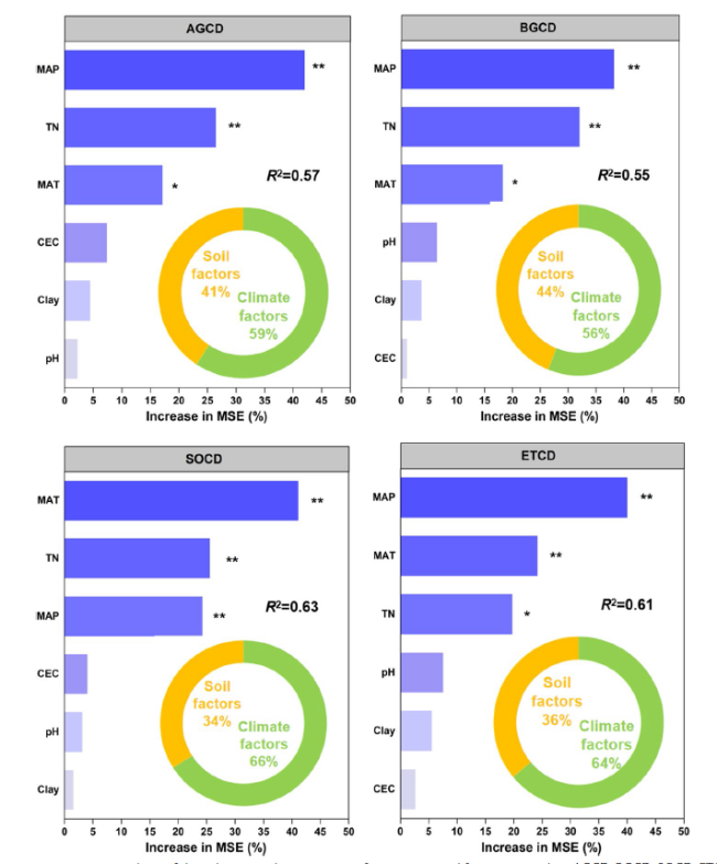
Fig. 7 The variation partitioning analysis of the relative explanatory rate of environmental factors to explain AGCD, BGCD, SOCD, ETCD. The circular rings mean the relative explanatory rate of soil and climate factors to AGCD, BGCD, SOCD, ETCD. The explained variability was calculated after 999 bootstraps. AGCD: above-ground carbon density; BGCD: above-ground carbon density; SOCD: soil organic carbon density; ETCD: ecosystem total carbon density; MAP: mean annual precipitation; MAT: mean annual temperature; pH: soil pH; TN: soil total nitrogen; CEC: soil cation exchange capacity |
Structural equation models (SEMs) were used to identify and quantify the driving factors to ecosystem C densities. The driving factors were divided into climate factors (MAT, MAP) and soil properties (i.e., pH, TN, clay and CEC) (Fig. 8). The final SEMs were built to describe the underlying flows of causality in driving factors to ecosystem C densities. Due to the high comparative fit index (CFI > 0.90), insignificant chi-square test (p > 0.05), and low root mean square error of approximation (RMSEA < 0.05), the verified SEMs showed the good model fit. According to SEMs, the C density reduced with MAT while increased with MAP. To be specific, climate conditions, especially MAP, increased with AGCD in all ecosystem types, which can thereby offset the direct decline effect on SOCD, finally leading to the positive effect on ETCD. By contrast, AGCD decreased with MAT in all ecosystem types, thus offsetting the increase effect on SOCD, and finally generating the negative effect on ETCD, except for farmland.
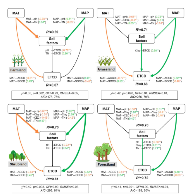
Fig. 8 Structural equation models (SEMs) depicting the multiple relations of ecosystem total carbon density (ETCD) with climate factors and soil properties, and the values are standardized coefficients of the models. The solid orange lines are the negative relationships, and the solid green lines are the positive relationships, and the solid black lines are no significant relationships, respectively. Arrows represent a directional influence of one variable upon another. The numbers beside the arrows are standardized coefficients. The thickness of the arrows is proportional to the magnitude of the standardized path coefficients or covariation coefficients. R2 stands for variation interpreted by variables, which is calculated after 999 bootstraps, and the significant level is set at α = 0.05, *p < 0.05, **p < 0.01. AGCD: above-ground carbon density; BGCD: above-ground carbon density; SOCD: soil organic carbon density; ETCD: ecosystem total carbon density; MAP: mean annual precipitation; MAT: mean annual temperature; pH: soil pH; TN: soil total nitrogen; CEC: soil cation exchange capacity |
4 Discussion
4.1 Spatial distribution of ecosystem C density
Based on the geostatistical analysis, the explanation for the proportions of the variances of ecosystem C density are more than 80% (R2 > 0.80, Table S6), so the fitting model is significant in terms of ecosystem C density. Previous studies have reported a high spatial heterogeneity in soil nutrients at large scale of Loess Plateau [50,51,52]. In this study, an exponential, spherical, or linear model with a sill were fitted using spatial auto-correlation for ecosystem C density (Table S6). Generally, there is a strong spatial auto-correlation with C/(Co + C) over 75%, moderate auto-correlation with 25-75%, and lower auto-correlation with less than 25% [51,52]. We found that the C/(Co + C) was over 50%, indicating that ecosystem C density had the obvious spatial auto-correlation. This is presumably due to the offset effects of spatial variances of ecosystem C density in different directions, and the complex terrain characteristics [53]. Further, the C/(Co + C) of above-ground C density (AGCD), below-ground C density (BGCD) and ecosystem total C density (ETCD) had a strong spatial auto-correlation, while SOC density (SOCD) had a moderate spatial auto-correlation, supporting the evidence that the spatially structured variance can account for ecosystem C density [54].
The kriging estimates could be mapped, to reveal the overall trend of the C density. In detail, the high ecosystem C density mainly located in the northwest and southwest parts of Loess Plateau (Fig. 2), and relatively low C density in the northern. This spatial distribution patterns reflected a gradually decreasing trend from southwest to northeast, roughly in line with Loess Plateau’s topographic feature, as well as differences in land use, forest management, economic and social development [39]. Furthermore, the SOCD generally increased with MAP, while it decreased with MAT [36,55]. Our findings showed that SOCD were higher in zones with MAT higher than 10 °C, and ETCD were obviously higher in zones with MAT lower than 5 °C (Fig. S3). It indicates that C is accumulated more in cold or moist ecosystems across the Loess Plateau. Generally, the AGCD and BGCD were remarkably higher across regions with MAP above 500 mm compared with those with MAP below 500 mm [6,56]. This is because that the higher MAP was due to higher vegetation growth rates, and therefore C input rates were higher in ecosystem [9,13,14,22].
The mean SOCD in this area was lower than the average of China [6], but higher than the average on the Loess Plateau [39]. Specially, forestland and grassland SOCD was higher than farmland (Fig. 5). Similarly, a meta-analysis indicated an increase of SOC by 19% and 53%, following farmland conversion to forestland and grassland [40]. Thus, the findings supported that the conversion from farmland to forestland/grassland increases soil C contents [17,18]. On the one hand, forestland and grassland soils had especially high organic C because of large litter and root input [57]. When these ecosystem converted to farmland, the organic C would be lost. On the other hand, plant biomass as returned nutrients to soil through above-ground litter and root debris, thus rapidly increasing SOC content as above-ground biomass increased [17,18,21].
4.2 Carbon stocks across the loess plateau
Due to the large scale of vegetation restoration projects since the early 1990s, the accurate assessments on C storage on the Loess Plateau were started [36,39,58,59,60]. However, the assessed size differed substantially among the early studies due to the limited field measurements [39]. Here, we made the statistics of C density and stocks on the Loess Plateau and China derived from various studies, and compared with our results (Fig. 4). A meta-analysis pointed out that the total C stock of the Loess Plateau is approximately 2.3 Pg [39]. In this study, the total C stock in forestlands, shrublands, grasslands, and farmlands is higher than Li et al. [39], but lower than Liu et al. [60]. The data, covering almost 6.5% territory in China, held around 1.5%-3.2% total SOC stocks (ranged from 89 to 192 Pg C) at 0-10 cm across the country [6,61]. The total C stock among which 30% was stored in soil (0-20 cm), 53% in above-ground biomass, and 17% in below-ground biomass. Consequently, the amount of C stored in roots (about 17%) is substantial and should be considered when assessing C stock.
For plant C stock, our data (1.51 Pg C) was higher than a meta-analysis over the Loess Plateau (0.44 Pg C) [39], and also was far below the average in China (from 6.1 to 53 Pg C) [61,62], because the Loess Plateau area is only one of the large-scale ecological restoration projects [6]. For soil C stock, previous studies conducted the assessment using soil profiles across the Loess Plateau [36,58,59]. However, due to the limited number of soil profiles and the fact that soil gravel was not excluded, the soil C stock estimation was quite large [36,58,59]. In fact, soil C stock of 0-20 cm was lower than those obtained by Li et al., (1.52 Pg) [39]; Fu et al., (1.64 Pg) [59]; Liu et al., (1.68 Pg) [36]; Xu et al., (1.07 Pg) [58]. In these previous studies, most of vegetation was artificially planted about 20 years, and the large root system is benefit to the soil C sequestration, then, the SOC storage generally increases with afforestation years [36,59]. Specially, the C stocks in the soil of grassland and farmland were higher than below-ground biomass, which is similar to the estimates for the continental China (3.9 Pg) [6], United States (3.0 Pg) [63] and Europe (3.5 Pg) [64]. However, higher SOC stock does not necessarily lead to greater ecosystem C stocks. For example, the C stocks in the soil of forestland and shrubland were lower than the biomass due to the “Grain-for-Green” project in China, which had built numerous forestland and shrubland regions [6,56]. As for these biomass, there was a quadratic equation relation between AGCD and BGCD (p < 0.05, Fig. S2). Hutchings and John [65] suggested that plants can adjust biomass partitioning to equalize growth limitations by essential resources, and thought that both ontogeny and environmental conditions exert influences on AGB and BGB partitioning, which is consistent with the optimal allocation hypothesis. In this case, plants adjust their growth strategy according to different environments, and in particular, tend to partition more biomass to root systems under more stressful, low-nutrient and harsh climatic conditions [66]. This made the parabolic regression between AGCD and BGCD on the Loess Plateau, and consequently, ecosystem C stocks can be substantially enhanced by fostering above-ground and below-ground C stocks.
The area-weighted mean AGCD and BGCD in forestland (72 Mg ha− 1), and grassland (1.0 Mg ha− 1) across the Loess Plateau (Fig. 5) were substantially lower than the global means [94 Mg ha− 1 in forestland and 7.2 Mg ha− 1 in grassland] [6,28,56]. Large-area young forests, extensive grazing and soil water limitation are the possible contributors of low C density of the Loess Plateau [32,33]. Most vegetation was artificially planted between 1990 and 2000, and the forest age was only about 20-30 years [39,40]. This relatively short period of time since vegetation restoration was not sufficient to develop the root system into the deep soil layers [21,67,68]. Almost 90% forests are aged below 60 years, and corresponding biomass is below 60 Mg ha− 1, obviously lower compared with that (105 ± 30 Mg ha− 1) in old forests (≥100 years) and mean of forests (200 Mg ha− 1) in China [69]. As these young and middle-aged forests gradually grow, the C sequestration of forestland on the Loess Plateau will increase [21,57,70]. In this case, future C sinks may surmount our estimates after forest areal expansion, vegetation restoration and protection and soil C increasing needs to be examined [71].
4.3 Effects of climate factors and soil properties on C density
We found the negative correlation between AGCD and MAT in forestland and grassland (Fig. 6), suggesting that the water stress rather than temperature limited plant growth in this area. We thought this result may be attributed to the high soil salinity, which is consistent with previous results [72]. However, BGCD is positively correlated with CEC. The CEC of a given soil can indicate how well some nutrients (mainly cations) could be bound to the soil. The improvement in soil CEC reflects a higher nutrient retention capability and a lower nutrient loss through leaching, which is beneficial for soil microbial activity and C sequestration [73]. For example, in sandy soil, SOC increased the CEC, and Oorts et al. [74] found that up to 95% of variation in CEC was attributed to SOC. Previous study also showed that some cations such as Ca2+ could play a role in stabilizing organic C in alkaline soils, because some cations can bridge negatively charged organic compounds together, forming organo-metal structures which protect SOC [75]. As for soil properties, the fine particles (clay and silt) reinforce organic matter retention due to their capacity of providing physical protection against microbial decomposition [16,67], and thus the significant correlation between SOC and clay content [16,37,67,76]. For example, Liu et al. [36] collected soil samples for over 380 sites on the Loess Plateau, and showed the general control of soil texture on the SOC density. Similar, Pearson correlation analysis revealed that clay content was an important factor influencing SOCD and ETCD (Fig. S3). The findings primarily revealed how clay and silt protect SOC. The high soil pH (> 8.0) reduced SOC accumulation through suppressing microbial activity and expediting the leaching of dissolved organic C in subsoil layer [56,63]. The lower pH forms increasing complexes with high-molecular weight organic compounds for binding aggregates, which is conducive to SOC stability [77]. Such improvement of aggregate stability increases SOC stability and accumulation.
According to the variation partitioning analysis, the total explained variance of climate factors to ABGD, BGCD, SOCD and ETCD were higher than soil properties (Fig. 7), and ETCD were dependent on MAT and MAP (p < 0.01). Moreover, the biogeographical pattern of ecosystem C density coincide with temperature and precipitation distribution patterns (Fig. 2), supporting our hypothesis that there was a critical role of climate factors in shaping the distribution of ecosystem C densities. Specially, climate factors influence ecosystem C accumulation by biotic processes related to vegetation productivity and organic matter decomposition [3,14,78,79]. These results also indicated the control of climate factors on ecosystem C density, supporting the results from Tang et al. [6] who revealed the intimate correlation between C density and climate: it reduced with temperature but increased with precipitation in China.
According to structural equation models, MAT exerted relatively large, direct, and negative effects on SOC stock (Fig. 8). MAT in this region decreased from the southeast to the northwest, and lower MAT reduced SOC turnover rates, causing an increase of SOC [16,36]. By contrast, higher MAT led to the faster SOC decomposition [80]. Generally, SOCD increased with MAP from the southeast to the northwest across the research area, because the higher MAP led to the higher soil moisture, which increases microbial metabolic activities and enzymatic activities, and thus formed relatively high SOC [36]. At specific precipitation level, SOCD reduced with MAP mainly because of the growing of soil respiration [81]. Nevertheless, MAT might increase SOC and offset the precipitation’s positive effect, which was obvious in farmland and grassland (Fig. 8). Similar, MAP was strongly related to AGCD, therefore counteracting the decreasing effect against SOCD. Comparatively, AGCD decreased with MAT in all ecosystem types, thus offsetting the increasing effect on SOCD, and finally generating the decreasing effect on ETCD, except for farmland.
5 Conclusions
The large-scale ecosystem C stocks and their driving factors were studied by the widespread field sampling across the Loess Plateau, to fill major gaps and uncertainties in the C stock estimations. The total ecosystem C stock was 2.8 Pg, among which 30% was stored in soil (0-20 cm), 53% in above-ground biomass, and 17% in below-ground biomass. Ecosystem C density decreased with MAT, while increased with MAP. In detail, climate factors (MAP, MAT) explained 59%, 56%, 66% and 64% of the total variance, while soil properties explained 41%, 44%, 34% and 36% of the total variance of above-ground C density, below-ground C density, SOC density, and total ecosystem C density, respectively. The findings supported the theoretical forecasts that on similar soils parent materials the large-scale patterns for ecosystem C density mainly come under climate control.
Abbreviations
BA:Basal area
DBH:Diameter breast height
BD:Bulk density
SOC:Soil organic carbon
AGCD:Above-ground carbon density
BGCD:Below-ground carbon density
SOCD:Soil organic carbon density
ETCD:Ecosystem total carbon density
AGCs:Above-ground carbon stock
BGCs:Below-ground carbon stock
SOCs:Soil organic carbon stock
ETCs:Ecosystem total carbon stock
MAP:Mean annual precipitation
MAT:Mean annual temperature
pH:Soil pH
TN:Soil total nitrogen
CEC:Soil cation exchange capacity
MSE:Mean squared error
SEMs:Structural equation models
RMSEA:Root mean square error
CFI:Comparative fit index
AIC:Akaike information criterion
Supplementary Information
The online version contains supplementary material available at https://doi.org/10.1007/s43979-023-00044-w.
Additional file 1: Fig. S1.The linear regression between SOC/SOCD in 0-10 cm and 10-20 cm. The gray area refers to the 95% confidence interval around the regression lines. All regression lines are significant at least at p < 0.05. Fig. S2. The parabolic regression between AGCD and BGCD. The gray area refers to the 95% confidence interval around the regression lines. Fig. S3. Mean ecosystem C density across the Loess Plateau depending on annual temperature and precipitation. Lowercase letters denote significant differences among ecosystem types; * and ** denotes significant differences within an individual temperature (p < 0.05, p < 0.01) (Duncan’s Multiple Range Test). The error bars represent ± one standard error.
Additional file 2: Table S1.The plant types of the study sites across the Loess Plateau. Table S2. The precision of the model of kriging interpolation for ecosystem C stocks. Table S3. The precision of the random forest model for ecosystem C stocks. Table S4. Summary of soil properties about ecosystems across the Loss Plateau of China. Table S5. Geostatistical parameters for soil factors across the Loess Plateau. Table S6. Geostatistical parameters for soil organic carbon (0-10 cm and 10-20 cm) and ecosystem carbon density across the Loess Plateau.
Acknowledgements
We sincerely thank the authors whose work is included in this work. We also thank the Editor, and three anonymous reviewers for their constructive comments that improved the quality of an earlier version of this manuscript. Scott X. Chang and Ann M. Logsdon polished the language.
Authors’ Contributions
YY: Writing—original draft, Writing—review & editing, Investigation, Formal analysis, Data curation. LLX: Project administration, Funding acquisition, Investigation. WF and ZPP: Project administration, Resources. XC and ZZK: Project administration, Resources, Investigation. ASS and WYQ: Resources, Investigation. YK: Supervision, Project administration, Writing—review & editing, Conceptualization, Investigation. The author(s) read and approved the final manuscript.
Funding
Open access funding provided by Shanghai Jiao Tong University. This study was funded by the National Natural Sciences Foundation of China (42107282), Comprehensive research on carbon sink survey of natural resources in typical areas of China (ZD20220133), Innovation Cross Team-Key Laboratory project of the Chinese Academy of Sciences, and the State Key Laboratory of Loess and Quaternary Geology, Chinese Academy of Sciences (No. SKLLQGPY2004).
Availability of data and materials
The data that support the findings of this study are available from the corresponding author upon reasonable request.
Declarations
Ethics approval and consent to participate
The manuscript is original and not submitted to other journal, all the results are without fabrication. The authors consent to participate in the manuscript.
Consent for publication
We agree to publish the work.
Competing interests
The authors have no competing interests to declare that are relevant to the content of this article.
All authors certify that they have no affiliations with or involvement in any organization or entity with any financial interest or non-financial interest in the subject matter or materials discussed in this manuscript.
