
1 Introduction
1.1 Flow fields for redox flow batteries
To mitigate the negative impacts of global climate change and address the issues of the energy crisis, many countries have established ambitious goals aimed at reducing the carbon emissions and increasing the deployment of renewable energy sources in their energy mix [1,2]. To this end, integrating intermittent renewable energies, such as solar and wind energies, into the grid has become a crucial challenge [3,4]. However, the inherent variability and unpredictability of these energy sources necessitate the deployment of energy storage systems [5,6]. Pumped hydro, compressed air, and electrochemical energy storage are among the most promising energy storage technologies, which can balance the mismatch between renewable energy generation and demand, thus contributing to a more sustainable and reliable energy supply [7,8,9,10]. Unlike pumped hydro and compressed air, electrochemical energy storage devices such as lithium-ion batteries and redox flow batteries (RFBs) are not limited by geology and geography. Even though lithium-ion batteries show high energy density, they may be unsuitable for large-scale applications due to the safety hazards [11,12]. Aqueous redox flow batteries (ARFBs), such as vanadium redox flow batteries (VRFBs), are intrinsically safe and have a long cycle life, which are regarded as promising technologies for large-scale energy storage [13]. Despite the promising potential of RFBs, their widespread implementation has been impeded by the high capital cost. To overcome this challenge, enhancing battery performance has been recognized as an efficacious strategy for reducing battery costs. Specifically, augmenting the power density at a given energy efficiency (EE) can potentially curtail the battery size, consequently diminishing the dimensions of associated components like graphite plates and membranes. Additionally, the improved EE can lead to higher electrolyte utilization (EU), thereby reducing the volume of electrolyte required during operation, which accounts for most of the capital cost in long-duration energy storage systems [14,15,16,17].
Generally, improving the battery performance requires reducing activation loss, ohmic loss, and mass transport loss [18]. Moreover, to achieve high system efficiency (SE), it is imperative to minimize the pumping work. As illustrated in Fig. 1a and b, a flow cell typically comprises graphite plates, porous electrodes and a membrane. The materials properties and cell architecture directly influence the battery performance. Traditionally, a “flow-through” cell structure, which is simple to manufacture, is commonly used in RFBs. In such a configuration, the electrolyte enters the active area from one side and flows through the whole length of the electrode. As a result, the flow-through structure always requires thick electrodes (usually larger than 3 mm) with small compression ratios to alleviate the large flow resistance and thus yield manageable pressure drops, which, however, leads to high ohmic resistance and low EE, especially at large current densities [19,20,21].
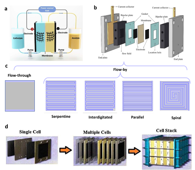
To circumvent this issue, a flow-by structure with flow channels grooved on the graphite plate was employed. The electrolyte is transported across the active area via the channels with a relatively low pressure drop, and the convection distance within the electrode is greatly shortened so that an ultra-thin electrode can be used to achieve lower ohmic polarization and enhanced electrochemical performance. For example, Aaron and Mench et al. adopted a zero-gap flow field (flow-by structure) with carbon paper electrodes, enabling the dramatic improvement of battery performance due to the significantly reduced ohmic loss, whose area resistance is measured to be only 0.5 Ω cm2, as compared to 3.5 Ω cm2 with flow-through configurations [25].
Till now, numerous typical flow patterns, including serpentine, interdigitated, parallel, and spiral structures, have been extensively researched [23,26,27,28,29,30,31], as illustrated in Fig. 1c. Each type of flow field has unique features in mass transport and pressure drop, thereby leading to distinct cell performances under different assembling and operating conditions. Serpentine and interdigitated flow fields are the most frequently studied and compared designs. It is found that the overall battery performance heavily depends on the balance between the electrochemical polarizations and pumping work [18].
More significantly, there exist many issues when scaling up the flow cell toward the stack-scale batteries. In engineering applications, the stack consists of several flow cells that have enlarged active areas, as shown in Fig. 1d. One challenge is that the applicable electrolyte flow rate in stacks is usually much lower than that in the lab-scale batteries for lowering the pressure drop and maintaining the airtightness [27,32,33], which leads to inadequate mass transport and large electrochemical polarization. Another challenge is that the pressure drop associated with the pumping work inevitably increases even with a low flow rate after scale-up due to the elongated flow channel and lengthened convection distance in electrodes. Therefore, rational designs of flow fields that can distribute the electrolytes uniformly at a minimized pressure drop are urgently needed to scale up the high-performance RFBs.
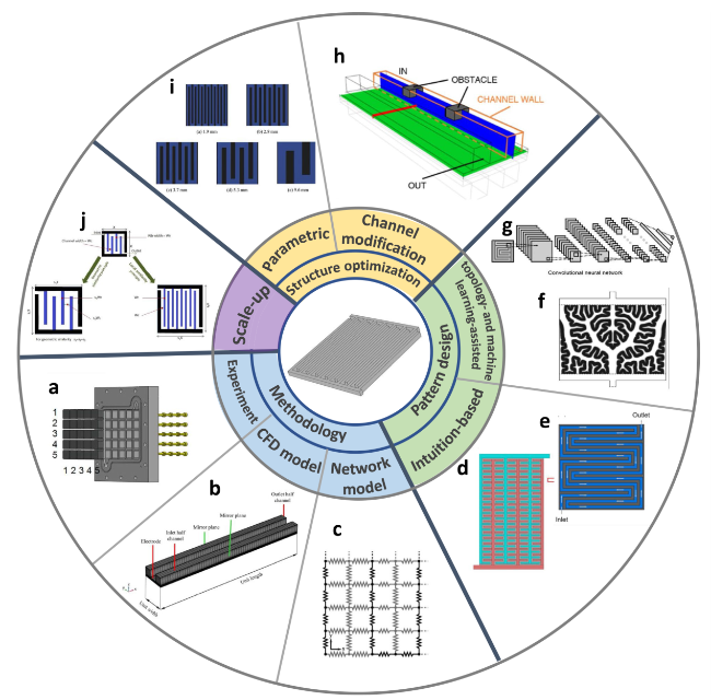
This review aims to comprehensively summarize the recent progress in developing flow fields in RFBs. We begin by discussing the critical issues related to flow field design, including mass transport and pressure drop. Then, we summarize the development of flow fields from various aspects, including methodology, flow field pattern design, structure optimization, and scale-up, as illustrated in Fig. 2. Numerical modeling is a technique used to simulate fluid flow, electrochemical reactions, and mass transport by representing them mathematically. It allows researchers to investigate the spatial and temporal distribution of key parameters and identify the optimization principle of flow fields without the need for physical experimentation. In pattern design, we not only compare flow-through and flow-by configurations with commonly adopted flow patterns, but also discuss novel flow pattern designs. Additionally, we summarize structure optimization by investigating geometric parameters and structure modifications. Finally, the critical challenges and strategies to scale up the flow fields are presented to provide perspectives for future flow field development. Overall, the review provides a comprehensive summary of recent progress in developing flow fields in RFBs, highlighting the importance of optimizing the design of flow fields for improving the performance and scalability of RFBs.
1.2 Critical issues in flow field design and optimization
1.2.1 Influence of flow fields on mass transport
Different from the static battery setup, in RFBs, the reactants are continuously pumped to the electrochemical cells while the products are removed from the cells, and the battery performance is significantly influenced by the mass transport process [22]. Specifically, mass transport is a complicated process that is coupled with electrolyte flow and electrochemical reactions. In addition, mass transport is affected by flow configurations, electrode/electrolyte properties, and assembling/operating conditions. Herein, we mainly discuss the influence of flow fields on mass transport. The flow-through and flow-by structures are the two main cell configurations to distribute electrolytes. In the flow-through configuration, the electrolyte directly flows into the electrode domain, while in the flow-by configuration, the electrolyte is transported in the flow channels and then convects into electrodes. Different flow patterns and geometric parameters lead to distinct velocity distributions, and a higher velocity magnitude contributes to lower concentration loss and higher ion transport flux. The ion flux of active species can be expressed according to the Nernst-Planck equation:
${{N}}_{{i}}=-{D}_{i}^{eff}\nabla {c}_{i}-{\mathrm{z}}_{i}{u}_{i}{c}_{i}F\nabla {\phi }_{l}+{u}{c}_{i}$
which constitutes the diffusion, migration and convection terms, where i indicates the species, ${D}_{i}^{eff}$ is the effective diffusivity, ${c}_{i}$, is the molar concentration, ${\mathrm{z}}_{i}$ is the charge number, ${u}_{i}$ is the mobility, F is the Faradaic constant, ${\phi }_{l}$ is the ionic potential in the electrolyte, ${u}$ is the electrolyte velocity. In a flow battery system, the diffusivity is relatively small while the convective item dominates the total ion flux. Therefore, higher concentration and velocity lead to a higher flux of ions [42]. In addition, the concentration overpotential can be expressed as [43]:
${\eta }_{c}=\frac{RT}{nF}\mathrm{ln}\left[1-\frac{i}{nF{k}_{m}{c}_{b}}\right]$
where ${\eta }_{c}$ is the concentration overpotential and ${c}_{b}$ is the reactant concentration in the bulk. Generally, the mass transfer coefficient can be evaluated by considering the velocity magnitude:
${k}_{m}=b{(\frac{v}{1 [m/s]})}^{n}\cdot 1 [m/s]$
where b and n are empirical constants, v represents the velocity magnitude of electrolyte in the porous electrode.
To determine the values of the constants, researchers calculate ${k}_{m}$ values at different electrolyte velocities and describe the correlation according to the fitting curve.
Specifically, ${k}_{m}$ values can first be calculated on the basis of the measured limiting current and basic parameters:
${k}_{m}=-\frac{v}{aL}ln(1-\frac{{I}_{lim}}{zF{t}_{e}W{c}_{i}^{in}v})$
where a is specific area, $L$, ${t}_{e}$ and $W$ are electrode length, electrode thickness and electrode width, respectively. ${I}_{lim}$ is measured limiting current. ${c}_{i}^{in}$ is the concentration of species in the electrolyte stored in the reservoir.
By adjusting the electrolyte flow rate, ${k}_{m}$ is calculated under a wide range of electrolyte velocities. A fitting curve is then generated to describe the dependence of mass transfer coefficient on electrolyte velocity, and the constants b and n in Eq. 3 are accordingly obtained [44].
It can be found that local concentration loss is directly influenced by the electrolyte velocity and concentration. In addition, the concentration of active species, as we can see from Eq. 1, is influenced by the velocity field. More sophisticated mass transport at the interface between electrolytes and electrodes is not discussed here. From the aspect of flow fields, the flow field pattern should be well-designed to lower the overall concentration overpotential. More significantly, the problem of non-uniform distribution of active species is exacerbated as the flow field is scaled-up, resulting in elevated concentration overpotential and performance degradation, which necessitates the implementation of effective and efficient scale-up strategies to mitigate the issue.
1.2.2 Influence of flow fields on pressure drop
In addition to mass transport, different cell configurations or flow patterns lead to different pressure drops and hence affect the pumping work. In fact, the pumping work constitutes a non-negligible part of the system power loss, which is dependent on the flow rate, cell architecture and dimensions. The flow field structure not only affects the flow resistance of channels, but also influences the electrolyte velocity and convection path within electrodes. The dependence of pumping work and VEpump on the pressure drop are given in Table 1. The pumping loss scales linearly as the pressure drop increases, and it affects both the charge and discharge processes.
Table 1 Evaluation parameters of RFBs |
| Parameter | Expression |
|---|---|
| Coulombic efficiency (CE) | $CE=\frac{\int I_{d}(t)dt}{\int I_{c}(t)dt}$ |
| Energy efficiency (EE) | $EE=\frac{\int E_{d}(t)I_{d}(t)dt}{\int E_{c}(t)I_{c}(t)dt} $ |
| Voltage efficiency (VE) | $VE=\frac{\int E_{d}(t)I_{d}(t)dt/\int I_{d}(t)dt}{\int E_{c}(t)I_{c}(t)dt/\int I_{c}(t)dt}$ |
| Pumping power (Wpump) | $W_{pump}=\frac{2q\Delta P}{\varphi} $ |
| Pump-based voltage efficiency (VEpump) | $VE_{pump}=\frac{E_{d,ave}I-W_{pump}}{E_{c,ave}I+W_{pump}} $ |
| System efficiency (SE) | $SE=\frac{\int(E_{d}(t)I_{d}(t)-W_{pump})dt}{\int(E_{c}(t)I_{c}(t)+W_{pump})dt}$ |
I denotes the current, and the subscripts d and c denote the discharge and charge process. E denotes the cell potential. q denotes the flow rate, ∆P denotes the pressure drop of the system, φ denotes the pump efficiency |
Hereinto, we first use the conventional flow-through configuration with the simplest flow process to demonstrate the effect of cell architecture and geometric dimensions. The pressure drop of the flow-through structure can be given by [18]:
$\Delta p=\frac{\mu q{L}^{2} }{ {t}_{e}K}$
${W}_{pump}=\frac{2\mu {q}^{2}{L}^{2} }{ {t}_{e}K\varphi }$
where $\mu$ is the electrolyte viscosity, $L$, ${t}_{e}$ and $K$ are the electrode length, electrode thickness and electrode permeability, respectively.
As illustrated in Eq. 6, the pumping work scales dramatically as the flow rate and convection distance increase. Therefore, there must be a critical flow rate over which the increased pumping work cannot be counteracted by the reduced electrochemical polarizations. In addition, compressing the electrode results in lower electrode thickness and permeability, thereby increasing the pressure drop of the battery system.
When the flow-by structures are applied to the RFBs, the convection distance within the electrode is greatly decreased since the electrolyte can be transported across the whole active area via the channels. Serpentine and interdigitated flow fields are two most widely used flow fields for distributing the electrolytes, while they have completely different characteristics and represent two types of flow field structures: one has connected inlet and outlet, and the other has disconnected inlet and outlet.
For the serpentine flow fields, the flow resistances of channels and electrodes between adjacent channels are in parallel relationship, hence only a portion of electrolyte penetrates into the electrode driven by the pressure difference of neighboring flow channels. Increasing the cross-sectional area of channels can lead to a lower pressure drop but increases the mass transport polarization due to the reduced penetration rate.
As for the interdigitated flow fields, the electrolyte flow enters the manifold from the inlet, disperses into inflow branch channels, flows into the electrode and across the under-rib region, then flows out through the outflow channels. Therefore, the interdigitated flow field is intrinsically a combination of several flow-through configurations in which all the electrolyte penetrates into the porous electrode [45]. Decreasing the channel width not only increases the flow resistance within channels, but also elongates the convection distance between inflow and outflow branch channels. In addition, the pressure drop in the main channels may increase considerably when scaling up the flow battery. It was found that a 400-cm2 cell with interdigitated flow field has a pressure drop of 0.05 MPa at a low flow rate of 2 mL min−1 cm−2, over 40% of which is induced by the flow resistance between the inlet pipe and branch channel end [46]. As a result, designing flow channels that can transport the electrolyte in a low pressure drop is an applicable approach to further improve the battery performance.
In addition to the conventional aqueous redox flow batteries, novel flow battery systems have emerged, including hypersaline slurry flow batteries and aqueous organic flow batteries. These systems exhibit unique kinetics and hydraulic properties compared to conventional electrolytes, necessitating the implementation of distinct flow fields.
For slurry flow batteries, different from conventional aqueous electrolytes which can be treated as Newtonian electrolyte with a constant viscosity, the slurry exhibits non-Newtonian behavior which can be described by the power law viscosity $\mu =K{(\dot{\gamma })}^{n-1}$,
Where $\dot{\gamma }$ is the shear rate, K and n are power law constants, and are fitted to be 5.72 and 0.18, according to the literature [47]. In addition, the electrolyte viscosity mainly ranges from 100-1000 cP [48,49,50,51], which is much higher than that of the conventional electrolyte (below 10 cP [27]). It is found that due to the increased flow resistance, the slurry flow battery is firstly demonstrated with only one straight flow channel [48,49]. Recently, zero-gap flow cells with serpentine flow fields were applied in the slurry flow cells [50,51]. Due to the high viscosity of the slurry electrolyte, the channel width needs to be increased to reduce the pressure drop. For conventional flow field, the channel width is relatively small (e.g., 1 mm [27]). In contrast, the channel width adopted in simulation of slurry flow batteries is 4.8 mm [47]. However, the investigation of flow fields is still in its initial stage since for slurry flow batteries, in addition to dramatically increased electrolyte viscosity, the construction of continuous electrolyte conductivity network is also critical for the steady operation. Currently, the cell is operated in continuous or intermittent mode. The flow field configuration, electrode properties, electrolyte properties under different operating conditions need to be further optimized and studied. Furthermore, due to the unique flow properties of slurry flow batteries, a numerical model that can accurately describe their behavior still needs to be established.
For aqueous organic RFBs, the viscosity and diffusion coefficient of aqueous organic electrolytes are compared with conventional electrolytes and found that both parameters fall within the same range [52,53,54,55,56,57,58]. Therefore, it is reasonable to assume that flow field design for aqueous organic RFBs can be borrowed from conventional RFBs, resulting in the use of flow-field-structured configurations such as serpentine and interdigitated setups. However, the specific geometric parameters of the flow field for a particular system may vary due to different hydraulic properties and kinetics of the electrolytes. Indeed, the properties of the electrolyte and the design of the flow field can affect mass transport and pumping loss from different aspects. In particular, viscosity directly impacts the flow of electrolyte through channels and electrodes, and higher viscosity can lead to greater pressure drop and pumping loss. Consequently, the degree of pumping loss in different systems can vary depending on the electrolyte’s viscosity. When it comes to mass transport, the ion flux is determined by a combination of convection, diffusion, and migration as shown in Eq. 1. The design of the flow field can directly impact the convection term in mass transport, while the ion diffusivity plays a significant role. In summary, while the flow field design for aqueous organic RFBs can be adapted from conventional RFBs, it is important to consider the different kinetics and hydraulic properties. The specific flow field design should take into account both electrochemical performance and pumping loss, which altogether are reflected in the system voltage efficiency.
2 Methodology
In this session, we elaborate on the experimental and simulation methods used in evaluating the flow fields, as shown in Fig. 3. Experimental tests are the most straightforward and persuasive approaches for evaluating and designing the flow fields. However, it is challenging to obtain the distribution of velocity magnitude and reactants concentration through conventional experimental methods. In some studies, the spatial variation in electrochemical performance has been preliminarily evaluated through modified battery setups. For example, Messaggi et al. manufactured a custom macro-segmented flow battery setup to export locally resolved electrochemical characterization. As shown in Fig. 4a, the whole active area with serpentine and interdigitated flow fields is divided into ten segments, with which the polarization curves of each segment can be exported separately. The characteristics of the typical flow fields are successfully revealed by the segmentation method, that is, for the serpentine flow field, the segments near the inlet have a higher limiting current density, while for the interdigitated flow field, the segments in the middle region exhibit larger electrochemical polarization [59]. Hsieh et al. exported the local current distribution by dividing the graphite flow field plate into several segments, as shown in Fig. 4b1. It was found that the design with segmented graphite plate can eliminate the effect of the in-plane current flow on the current density distribution, and the corresponding results of different stages are presented in Fig. 4b2 and b3. The current density close to the outlet significantly decreases at the end of the discharging process [34].
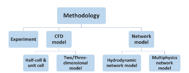
Fig. 3 Outlines of methodology for evaluating flow fields |
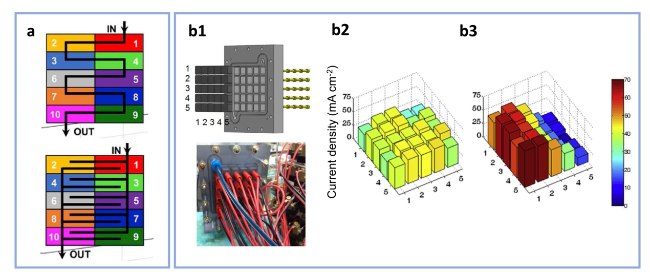
Fig. 4 a Schematic diagram of the segmented flow fields (reproduced with permission from Ref. [59]). b1 Schematics and photos of a graphite flow field plate divided into 25 segments. Current density distributions of the segmented graphite flow field plate at (b2) the beginning of the discharging process, b3 the end of the discharging process with a current density of 40 mA cm−2 (reproduced with permission from Ref. [34]) |
Even though, conducting the experiments consumes a lot of resources when scaling up the flow battery and systematically investigating the effect of geometric parameters. Modeling the flow battery is an effective way to describe the flow distribution with a relatively low cost. Among numerous implemented numerical models, a three-dimensional model coupling fluid flow, mass transport and electrochemical reactions accurately describes a flow cell [60,61,62,63,64,65]. As shown in Fig. 5a1, the computational domain comprises the electrodes and flow channels on both the negative and positive sides, which is separated by the membrane. Such a model can provide the visual distribution of key parameters for illustrating the influence of flow field designs. Figure 5a2 presents the contours of V2+ ions concentration at the mid-plane in the electrode for serpentine, interdigitated and rotary serpentine flow fields. The flow cell with novel flow field exhibits an obviously higher reactant concentration, which is in accordance with the superiority of rotary serpentine flow field in electrochemical performance [60]. Considering that the flow fields affect the overall battery performance by influencing the fluid flow and mass transport process, the flow distribution on both sides is similar and independent on the membrane. Therefore, some researchers conduct simulations for the positive and negative sides separately. Correspondingly, the computational domain is only comprised of an electrode and flow channels on one side, as depicted in Fig. 5b [61]. When studying the geometric parameters of interdigitated channels, researchers typically use a unit domain that includes only a small number of flow channels. This is because the flow behaviors from the inflow branch channel into adjacent outflow channels are similar, as shown in Fig. 5c [62].
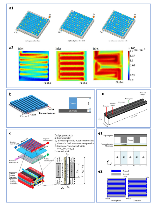
Fig. 5 a1 Three-dimensional computational domain of cells with serpentine flow field, interdigitated flow field and rotary serpentine flow field. a2 Distributions of V2+ ions concentration in the mid-thickness plane of the electrode with different flow fields at 0.8 SOC (reproduced with permission from Ref. [60]). b Schematic of half-cell three-dimensional computational domain and cross-sectional view of flow channel and electrode (reproduced with permission from Ref. [61]). c Schematic of computational domain for the unit interdigitated flow field (reproduced with permission from Ref. [62]). d Schematic view of a single RFB cell with interdigitated flow field and two-dimensional computational domain (reproduced with permission from Ref. [66]). e1 Schematics of flow field structure and computational regions. e2 Schematics of two-dimensional computational domain with two regions for interdigitated and serpentine flow fields (reproduced with permission from Ref. [23]) |
Moreover, the two-dimensional model is also widely used based on the characteristics of different channels to further reduce the computational cost. Specifically, as shown in Fig. 5d, adopting the cut plane perpendicular to the flow channel is commonly used to describe the convection process of interdigitated flow fields [66]. Such simplification applies to studying the effect of dimensions and flow channel modifications of the interdigitated flow fields, while an in-plane two-dimensional model is needed when comparing different flow field configurations. Zhang et al. constructed two regions to represent the flow channels and porous electrodes on one of the negative and positive sides. Figure 5e presents the schematics of flow field structure and simplified computational domain for serpentine and interdigitated flow fields. It is worth noting that the channel depth and electrode thickness are taken into account to calculate the velocity magnitude and maintain the mass conservation at the boundary of two regions [23].
Another modeling strategy for flow batteries is to simulate the segmented channels/electrodes with connected flow resistances. In most studies, the flow cell region is divided into segments, and each segment has similar geometric dimensions. Figure 6a illustrates the segmented hydrodynamic network diagram developed by Latha et al. for a 4-pair interdigitated flow field. In this diagram, the flow resistances of the inflow branch channel and outflow branch channel are connected through the flow resistances of the electrodes [67]. Ha et al. proposed a two-layer hydrodynamic network to describe the fluid flow in channels and electrodes in detail. Figure 6b shows the schematics of the flow resistance network and the corresponding grid setting of the model using finite element method (FEM) for the serpentine flow field. The flow resistances connecting the two layers represent the flow process in through-plane direction. The network model captures the trend of pressure drop predicted by FEM model. However, compared to the widely used FEM, the network model provides pressure and velocity distributions with a relatively low resolution [35]. Besides, the network model can be further combined with the description of mass transport and electrochemical reactions for presenting a more comprehensive evaluation of flow cells. As shown in Fig. 6c1-c3, Jiao et al. constructed the flow resistance network according to the electrolyte flow pattern and supplemented the species transfer caused by the convection, diffusion between adjacent segments as well as the charge transfer network. Results of the coupled model in Fig. 6c4 show good agreement with the experimental data and numerical results (from FEM model) in both charge-discharge voltages and pressure drops under varying compression ratios. More importantly, the network model provides a transient simulation method with a low computational cost, which successfully predicts the significant capacity decay at low current densities due to the crossover, as depicted in Fig. 6c5 [68].
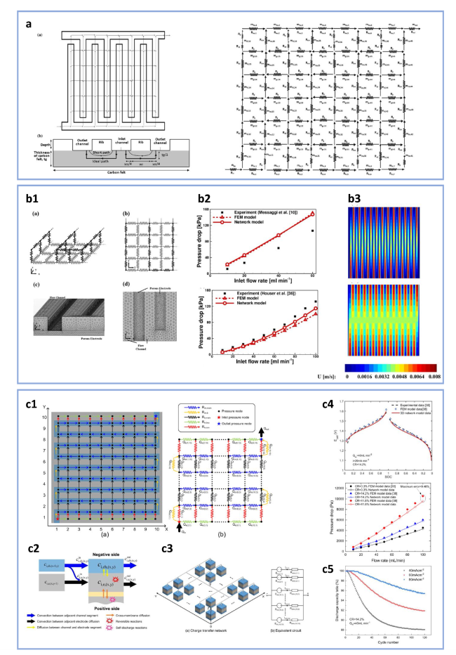
Fig. 6 a Schematic of a 4-pair segmented interdigitated flow field, transverse length through the porous electrode and hydrodynamic network diagram (reproduced with permission from Ref. [67]). b1 Computational grids for an RFB cell with serpentine flow field used in the two-layer hydrodynamic network model and FEM model. b2 Comparison of pressure drops obtained from the network model with those from experiments and FEM model with serpentine flow field. b3 X-direction velocity distribution of the FEM model (up) and two-layer network model (down) within the porous electrode with serpentine flow field at 20 mL min−1 (reproduced with permission from Ref. [35]). c1 Schematic of electrolyte flow pattern and corresponding flow resistance network. c2 Schematic of species transfer caused by the diffusion, convection between adjacent segments. c3 Schematic of charge transfer network and equivalent circuit. c4 Comparison of charge-discharge curves and pressure drops obtained from the network model with those from experiments and FEM model. c5 Predicted discharge capacity ratio at different current densities (reproduced with permission from Ref. [68]) |
To sum up, modeling the flow cell helps to systematically understand the dependence of battery performance on the flow field design and optimize the flow field structure. The adoption of unit cell and two-dimensional models with reasonable justifications is an applicable solution to further reduce the computational cost. Furthermore, the construction of network model provides another strategy to investigate the fluid flow and mass transport process by describing the cell with several segments. Compared to the FEM models, the network model can reduce the computational cost with little sacrifice in accuracy due to fewer computational nodes, resulting in its potential in multiple-parameter optimization, describing the transient process and modeling the stack-scale batteries.
3 Flow field pattern design
3.1 Classic flow field patterns
The comparison between different cell configurations is influenced by operating and assembling parameters, including electrode materials, flow rate, operating current density, as well as the geometric dimensions of a typical flow field, while the effects are reflected in the activation, ohmic and concentration overpotentials. Typically, the flow-through or flow-by cell structure affects the electrochemical performance by influencing the electrolyte distribution in the electrode and the cell ohmic resistance, which is indicated by the cell charge/discharge voltage or VE. However, the influence on pressure drop should be considered when evaluating different cell configurations; hence the SE and VEpump are the other essential indicators that consider the pumping work. Therefore, it’s hard to make a conclusion when comparing different cell structures without considering the geometric parameters, operating conditions, and indicators, that’s the reason why different and even contradictory results are presented from the literature.
3.1.1 Flow-through and flow-by architecture
In this section, we will first compare the battery performance of flow-through and flow-by structures. The flow-through configurations are the earliest adopted cell architectures in RFBs, and there are mainly two types of flow-through configurations. In the first configuration, the electrolyte enters the electrode and exits from diagonal corners [69] and the second type employs inlet and outlet distribution channels on two sides [30], as shown in Fig. 7a1. Typically, the electrolyte distribution in the second type flow-through configuration exhibits higher distribution uniformity than the first type. Zheng et al. numerically optimized the flow-through structures by introducing guidance and distribution channels at inlets and collection channels at the outlets (corresponding to the two types of flow-through structure). As shown in Fig. 7a2, such a design enables the plug flow of electrolytes, which leads to a more uniform distribution in the flow-through structure [70]. The flow-by-structured configurations engrave flow channels on the graphite plate to distribute electrolytes, and then the electrolytes convect into the porous electrode. The electrodes are tightly attached to the flow fields without gaps, therefore, such configuration is also called “zero-gap” architecture.
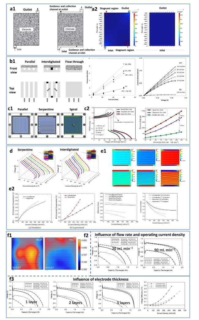
Fig. 7 Comparison between conventional cell configurations. a1, a2 Different types of inlet design for flow-through configurations (reproduced with permission from Ref. [70]), b1, b2 comparison between parallel, interdigitated and flow-through configurations (reproduced with permission from Ref. [71]), c1, c2 comparison between parallel, serpentine and spiral configurations (reproduced with permission from Ref. [29]), d local polarization curve measurement for serpentine and interdigitated flow fields (reproduced with permission from Ref. [59]), e1, e2 numerical comparison between serpentine and interdigitated flow fields (reproduced with permission from Ref. [23]), and f1-f3 influence of operating conditions and electrode properties on the comparison between serpentine and interdigitated flow field (reproduced with permission from Ref. [27]) |
We will compare the battery performance with and without flow fields from the aspect of hydraulic and electrochemical performances. As shown in Fig. 7b2, since all the electrolyte transports inside the porous electrodes, the electrolyte velocity is relatively high and convection distance is rather long, which results in a high pressure drop in the flow-through structures [69]. As for the influences on the electrochemical performance, the structures with and without flow field affect the cell ohmic loss and the electrolyte distribution inside the electrodes. As discussed in the introduction part, the flow-by configuration enables the adoption of thin electrodes, which significantly reduces the ohmic loss. Xu et al. compared the RFB performance with and without flow fields. The flow-through structure can lead to a more uniform distribution in the through-plane direction, while the flow-by configuration leads to a more uniform in-plane distribution, The through-plane electrolyte supply is mainly from the convection and diffusion, and such transport can be enhanced through increasing the flow rates. Therefore, the battery with serpentine flow fields shows a higher discharge voltage and, thereby, a higher VE at high flow rates [72]. Xu et al. also applied a numerical model to compare different flow configurations, and results show that the flow-field-structured batteries exhibit a higher electrolyte distribution uniformity than the flow-through structure [26]. Since the electrolytes are directly pumped into the electrodes without the guidance of flow channels over the convection path, the electrolyte may be maldistributed inside the electrode in the flow-through structure, which leads to poor battery performance, especially when the electrode active area is enlarged, as reported in Ref. [69]. Overall, the flow field configurations can reduce the pressure drop and lead to more uniform distribution of electrolyte. More importantly, there leaves great flexibility and space to design the flow patterns, adjust the geometric parameters in the flow field structures.
3.1.2 Flow field configurations
Characteristics of different flow fields In this section, we will compare the most widely studied flow fields, which include parallel, serpentine, interdigitated, and spiral flow fields. These flow fields have been extensively studied in fuel cells [73,74,75]. However, there are fundamental differences in transport properties (e.g., the diffusivity of the fluids) between liquid electrolytes in RFBs and the gas in fuel cells. The transport mechanisms and optimal flow field design for RFBs need to be thoroughly investigated. As depicted in Fig. 7b, the parallel flow field consists of parallel channels, all of which are connected to both the inlet and outlet manifold. Typically, this flow field shows the lowest pressure drop but also weak under-rib convection, leading to nonuniform distributions of electrolytes [67]. The interdigitated flow fields also exhibit parallel flow channels, but the branch channels are alternately connected with the inlet or outlet manifold, forming two disconnected parts. The electrolyte enters the inflow channel and is forced into the electrode, then flows out from the outflow channels, leading to increased uniformity of electrolyte distribution. The inlet and outlet of the serpentine and spiral flow field are connected by one channel but arranged in different path configurations.
Both the hydraulic and electrochemical performance of different flow fields have been studied. MacDonald et al. modeled the flow distribution and pressure drop within the flow-through, parallel and interdigitated flow fields. The hydrodynamic models show that the flow-through structure suffers from excessive pressure drop while the parallel flow field shows the lowest pressure drop and poor penetration of the electrolyte into the electrodes. In addition, optimizing the dimensions and geometric parameters of the interdigitated flow field can yield both high performance and lower pressure drop [76]. In addition to the hydrodynamic models, Darling et al. experimentally compared flow-through, parallel, and interdigitated designs assembled together with graphite felt or carbon paper electrodes. The cell with parallel flow fields shows lower performance even at relatively high flow rates due to the low penetration rate of electrolytes into the electrodes [71]. Huang et al. compared the parallel, serpentine, spiral flow fields using a multiphysics model. The cell with spiral flow fields shows the smallest voltage loss and, therefore, higher VE than the other two types of flow fields. However, the spiral flow fields have longer flow channels, which leads to increased pumping loss and hence a lower VEpump [29] (Fig. 7c). Due to the weak convection of the parallel flow field and the large flow resistance of the spiral flow field, these two types of flow fields receive the least research interest, while the serpentine and interdigitated flow fields are the most widely researched through both the numerical simulations and the experimental investigations.
Comparison between serpentine and interdigitated flow fields under different working conditions The serpentine and interdigitated flow fields are the most widely used configurations in RFBs. However, the characteristics of electrolyte flow in these two types of flow fields are quite different. Since the inlet and outlet are connected in the serpentine flow field, the electrolyte can preferentially transport in the channels or in the electrodes, which are decided by the pressure difference between adjacent channels. In contrast, the channels in the interdigitated flow fields are not connected. The electrolyte is distributed from the manifold to the inflow branch channels, then transported through electrodes via under-rib convection, and finally collected through the outflow branch channels and the manifold. Therefore, due to the distinct features of the two types of flow fields, both the pressure drop and electrolyte distribution in the two flow patterns are quite different. From the pressure drop aspect, a large proportion of the pressure drop in the interdigitated flow fields comes from the manifold [46]. In many cases, the pressure drop of interdigitated flow fields is smaller than the serpentine pattern due to the split electrolyte and shorter flow distance in branch channels. However, the pressure drop in the interdigitated flow field sharply increases when the electrode with lower permeability is used. From the electrolyte distribution aspect, the non-uniformity of reactant distribution in the serpentine flow field mainly comes from two parts. Firstly, the reactants are continuously consumed along the direction from inlet to outlet. Therefore, even though the velocity distribution under different ribs is similar, only the electrolyte near the inlet is rich in reactants and regions near the outlet usually demonstrates higher mass transport polarization. Secondly, the velocity under one rib is not uniform due to the weak convective regions at the turns of the pattern, since the electrolyte penetration into electrodes is driven by the pressure gradient in the two neighboring channels. In addition, the non-uniformity of electrolyte distribution in the interdigitated flow field also comes from two parts. Firstly, the flux of electrolytes in different branch channels is uneven. Secondly, the electrolyte velocity varies along a single branch channel. Messaggi et al. adopted a macro-segmented flow battery setup to perform locally resolved electrochemical characterizations. The local polarization curves corresponding to the different segments in serpentine and interdigitated flow fields reveal that the single serpentine channel shows decreased electrochemical performance from the inlet to the outlet, while the interdigitated configuration is limited in the central region of the active area, as shown in Fig. 7d [59]. It is difficult to determine which type of flow field, either serpentine or interdigitated, leads to better battery performance due to their distinct features in pressure drop and electrolyte distribution. The comparative conclusion may vary depending on the operating and assembling conditions.
Zhang et al. built a two-dimensional model and compared the serpentine and interdigitated flow fields with an active area of 9 cm2. The simulation results reveal that the interdigitated flow field shows a lower pressure drop due to the shorter channel length and a more uniform distribution of electrolytes than the serpentine configuration [23], as shown in Fig. 7e. Actually, the battery performance with serpentine and interdigitated flow fields may vary under different scales. Kumar et al. found that the comparative results get reversed for the serpentine and interdigitated structures with different active areas. On a 100 cm2 scale, their experimental results demonstrate that the serpentine flow fields show the highest electrochemical performance and the lowest pressure drop. However, on a smaller scale of 80 mm × 51 mm, the interdigitated flow fields show higher power density and less pressure drop. Such phenomenon is explained by the flow maldistribution that occurred when the interdigitated flow field is scaled-up [69]. In addition to the reversed battery performance induced by the scales, a more complex interplay between cell architecture and electrode properties and operating conditions is investigated by Houser et al., as shown in Fig. 7f. The interdigitated flow field outperforms the serpentine structure with a low flow rate of 20 mL min−1 and a thin electrode, but the battery performance with the serpentine structure can match that with the interdigitated at increased flow rates (90 mL min−1) and thicker electrodes. The interdigitated flow fields exhibit enhanced convection of electrolytes compared with the serpentine configurations since the electrolytes are forced into electrodes for the interdigitated architecture. Therefore, enhanced convection leads to better performance of the cell with interdigitated flow fields at low flow rates, however, the difference between flow fields is minimized at increased flow rates [27]. A similar conclusion was also reported in the work that Houser et al. compared serpentine, interdigitated, and flow-through structures with guidance channels [30].
It is noteworthy that cell size plays a critical role in influencing the performance comparison between cells with and without flow fields, as well as different flow patterns. During scale-up, pumping loss constitutes a significant portion when evaluating cell performance, and VEpump serves as a more comprehensive indicator in this regard. Owing to the distinct features of various cell configurations and their impact on mass transport and pressure drop, different flow configurations may necessitate distinct scale-up strategies, which will be discussed in greater detail in subsequent sections.
3.2 Novel flow field patterns
Previous studies have extensively examined conventional flow fields under various assembling conditions, operating conditions, and scales. However, there are still many issues in engineering applications. For instance, when applying flow fields to scaled-up batteries, cells with serpentine flow fields experience poor electrochemical and hydraulic performance due to elongated flow distance and uneven distribution of reactants. In cells with interdigitated flow fields, the increase in the number of channels results in uneven distribution of electrolyte into branch channels, which consequently leads to higher mass transport polarization. To enhance battery performance while minimizing pressure drop, several new flow field patterns have been proposed recently. In this section, we summarize the intuition-based designs of flow fields, which involve adjusting conventional flow channels such as serpentine, spiral, interdigitated, and parallel flow fields. However, optimizing conventional designs through trial-and-error approaches and limited human intuition can limit battery performance. Therefore, topology optimization and machine learning are introduced to generate irregular flow channels and facilitate high-throughput screening of flow field designs. The design process and results of optimization using new methods will also be presented, as shown in Fig. 8.
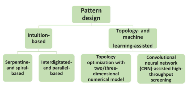
Fig. 8 Outlines for pattern design of flow fields |
3.2.1 Intuition-based flow field pattern design
Novel patterns based on serpentine and spiral flow field
Scaling up the flow cell with serpentine flow field usually suffers from the large pressure drop due to the excessively long flow distance in channels. Applying the split design to serpentine flow fields is regarded as an effective method to lower the pressure drop and maintain the even electrolyte distribution by decreasing the flow distance within each flow channel [23,77,78,79]. Gundlapalli et al. proposed several novel patterns including enhanced cross-flow serpentine and flip-flop serpentine flow fields, as shown in Fig. 9a. The adoption of flip-flop serpentine flow field greatly shortens the flow distance within the active area and reduce the system pressure drop compared to the conventional serpentine flow field. Additionally, the uniform electrolyte distribution leads to the timely replenishment of reactants, thereby improving the SE by over 2% [80].
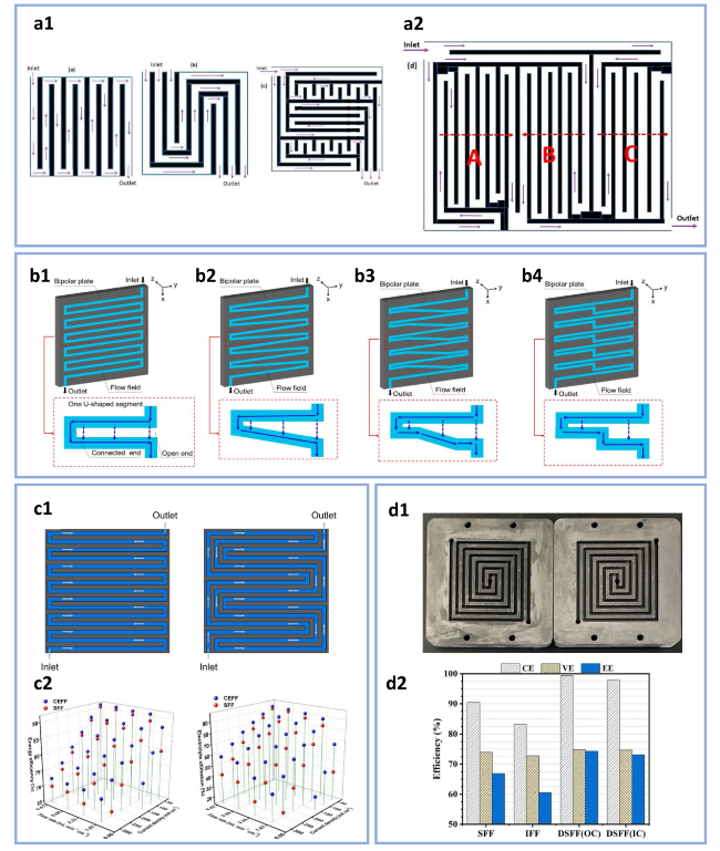
Fig. 9 Schematics of (a1) single serpentine flow field, three-parallel serpentine flow field, enhanced cross-flow serpentine flow field and (a2) flip-flop serpentine flow field (reproduced with permission from Ref. [80]). Schematics of (b1) conventional serpentine flow field, b2 serpentine flow field with the sloping channels, b3 serpentine flow field with the partially sloping channels and b4 serpentine flow field with the stepwise channels (reproduced with permission from Ref. [81]). c1 Schematics of conventional serpentine flow field and repatterned convection-enhanced flow field. c2 EE and EU with two flow fields under different flow rates and current densities (reproduced with permission from Ref. [36]). d1 Schematics of double spiral flow field with inlet/outlet at the center. d2 Efficiencies of the VRFBs with different flow fields (reproduced with permission from Ref. [82]) |
Other than the application of split channels, some novel configurations were also developed to improve the mass transport of the serpentine flow field. As previously mentioned, the mass transport polarization of serpentine channels is partially caused by the non-uniform velocity distribution under one rib. For the adjacent flow channels, the pressure difference at the connected end is nearly zero, while that at the open end is large due to the longer flow distance. Based on this, Sun et al. proposed three distinct manners (by introducing sloping channels, partially sloping channels and stepwise channels) for making the pressure gradient on the two sides of the rib uniform, as shown in Fig. 9b. By using the modified serpentine flow fields, the SE with pumping consumption considered is improved by about 4% compared to that with the conventional serpentine flow field at 100 mA cm−2 and 30 mL min−1 [81]. In some studies, researchers still use straight channels but rearrange the flow path to improve the uniformity of electrolyte distribution. Xu et al. were the first to propose a convection-enhanced flow field by tailoring the flow paths based on the conventional serpentine flow field in fuel cells. The pressure difference between adjacent channels is significantly increased due to elongated flow distance via channels [83]. Such a design was then introduced to RFBs and expected to reduce the electrochemical polarization since the mass transport of liquid electrolyte is more dependent on convection (Fig. 9c). Experimental results show that the EE with new flow field adopted is enhanced by 10% as opposed to that with conventional serpentine flow field, which can be attributed to larger convection speed and more uniform reactants distribution in electrodes [36]. Lu et al. numerically compared the convection-enhanced flow field with conventional serpentine and interdigitated flow fields based on the mass transport polarization and pressure drop. Although the cell with convection-enhanced flow field exhibits higher pumping consumption than that with interdigitated flow field, the new flow field still outperforms the other two structures in overall SE due to its significant advantage in reducing the mass transport polarization [60]. Generally, both the serpentine and spiral flow fields have connected inlet and outlet. In the study of Yang et al., the conventional spiral flow field shows inferior electrochemical performance due to the weak convection near the center of electrodes. To circumvent the issue, they developed two double spiral flow fields with outlet and inlet at the center, respectively, as shown in Fig. 9d. With the same pumping power, the application of the two novel designs improves the EE by 7.40% and 6.21% as opposed to the serpentine flow field [82].
It is worth noting that although some patterns are proposed with lab-scale active areas, the design principle still works for stack-scale batteries. Specifically, the pumping consumption accounts for a more significant proportion of power loss during the scale-up, which can be effectively mitigated by splitting channels. Moreover, the non-uniform electrolyte distribution becomes even more severe due to the elongation of flow distance. Enhancing the under-rib convection is always promising to improve the electrochemical performance of batteries at any scales.
Novel patterns based on interdigitated and parallel flow field Different from the serpentine flow field in which the electrolyte flow across the whole length of the flow channel, interdigitated flow field usually has a shorter flow distance since the electrolyte is distributed into branch channels from the inflow main channel and flows out directly via the outflow main channel after the convection process. However, it is still found that the pumping consumption may increase considerably when the cell scales up, and the pressure drop between the inlet pipe and distribution channel end accounts for 42% of the total pressure drop in a 400-cm2 cell [46]. Therefore, a hierarchical interdigitated flow field, which has independently regulated channels to lower the pumping loss and further enhance the mass transport, was proposed. Specifically, the main channel and primary branch channels with large sectional areas are designed to transport the electrolyte across the entire length of the active area, and the secondary branch channels with a small sectional area serve to inject the electrolyte into the adjacent electrode with a relatively high velocity to ensure good mass transport, as shown in Fig. 10a. Accordingly, experimental results show that the pumping loss is reduced by 65.9% and the VEpump is increased from 73.8% to 79.1% at 240 mA cm−2 and 3.0 mL min−1 cm−2 when the traditional interdigitated flow field is replaced by hierarchical interdigitated flow field [18]. Differently, Guo et al. proposed a bifurcate interdigitated flow field to alleviate the pumping consumption. As shown in Fig. 10b, the electrolyte is divided equally through hierarchical bifurcate channels outside the active area before entering the branch channels, which reduces the pressure drop during the electrolyte distribution/collection processes and maintains the uniform distribution of reactants. As a result, the pumping consumption is reduced by 45% with an active area of 105 cm2, hence the VEpump increases from 69.95% to 73.10% at 250 mA cm−2 and 2.4 mL min−1 cm−2 [84].
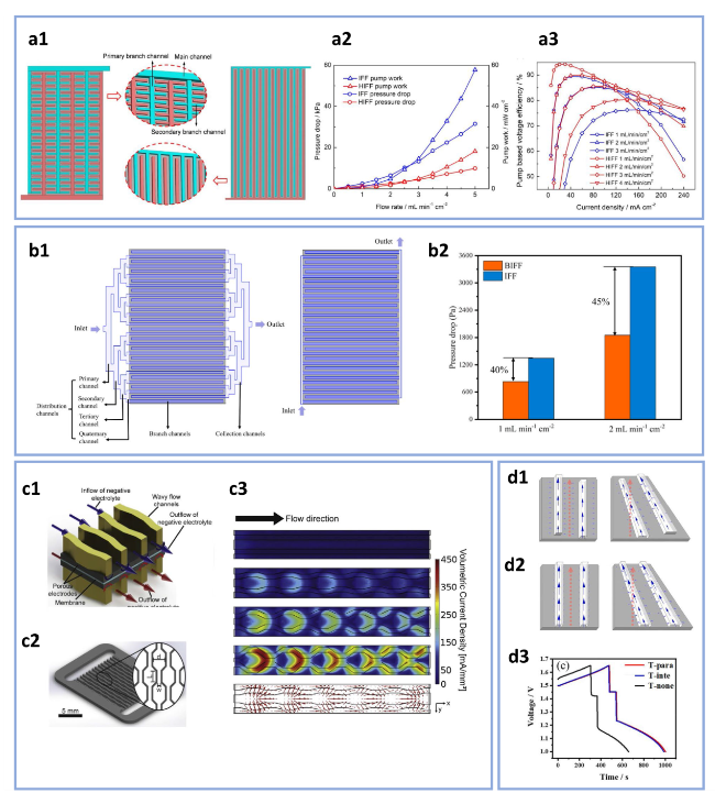
Fig. 10 a1 Schematics of the hierarchical interdigitated flow field and conventional interdigitated flow field. a2 Pressure drop and specific pumping loss of VRFBs with different flow fields. a3 VEpump of the VRFBs with different flow fields (reproduced with permission from Ref. [18]). b1 Schematics of the bifurcate interdigitated flow field and conventional interdigitated flow field. b2 Pressure drops of VRFBs with bifurcate interdigitated flow field and conventional interdigitated flow field (reproduced with permission from Ref. [84]). c1 Illustration of a section of the corrugated wall fluidic network. c2 Design of the 3D-printed fluidic network. c3 Volumetric current density distribution within the electrode and velocity arrows of cells with straight channels and corrugated channels (reproduced with permission from Ref. [85]). Schematics of rectangular flow field and trapezoid flow field with (d1) parallel channels and (d2) interdigitated channels. d3 Discharge curves of batteries with different flow fields at 200 mA cm−2 (reproduced with permission from Ref. [86]) |
Compared to the interdigitated flow field, the inflow and outflow main channels of parallel flow field are directly connected by branch channels, thereby leading to a low pressure difference between adjacent channels and weak under-rib convection. Therefore, Lisboa et al. replaced the straight parallel channel with corrugated channel systems, which employ periodic throttling of the flow to optimally deflect the electrolytes into the porous electrode, as shown in Fig. 10c. An improvement of up to 102% in net power density is obtained even with the adverse effect of increased pumping work [85].
Except for the optimization of flow field configurations, conventional flow fields are also applied to non-rectangular active area for improving the battery performance. For example, the trapezoid flow field shows great superiority in enhancing mass transport and improving the VE compared to the conventional rectangular flow field [87]. However, the relatively uneven distribution of electrolyte flow can still occur in the four corners of the trapezoid region. Hence the radial oriented quasi-parallel and quasi-interdigitated channels were applied to trapezoid flow fields, as shown in Fig. 10d. The introduction of channels improves the spatial distribution uniformity of electrolyte and accelerates the fluid velocity in electrodes, and thus reduces the polarization and increases the rate capacity of RFBs [86]. The comparison of flow batteries with novel flow field patterns and classic low fields is summarized in Table 2.
Table 2 Brief description of novel flow fields performance |
| Author | Active area and operating conditions | Flow field | Battery performance |
|---|---|---|---|
| Gundlapalli et al. [80] | 900 cm2, 120 mA cm−2, 0.6 mL min−1 cm−2 | Serpentine | 67.6% SE |
| Flip-flop serpentine | 69.5% SE | ||
| Sun et al. [81] | 25 cm2, 100 mA cm−2, 30.0 mL min−1 | Serpentine | 65.1% SE |
| Stepwise serpentine | 68.9% SE | ||
| Wei et al. [36] | 9 cm2, 250 mA cm−2, 1.67 mL min−1 cm−2 | Serpentine | 65.3% EE |
| Convection-enhanced | 75.3% EE | ||
| Lu et al. [60] | 100 cm2, 40 mA cm−2, 1.2 mL min−1 cm−2 | Serpentine | 81.6% VEpump |
| Interdigitated | 84.9% VEpump | ||
| Rotary serpentine | 86.0% VEpump | ||
| Zeng et al. [18] | 40 cm2, 240 mA cm−2, 3.0 mL min−1 cm−2 | Interdigitated | 73.8% VEpump |
| Hierarchical interdigitated | 79.1% VEpump | ||
| Guo et al. [84] | 105 cm2, 250 mA cm−2, 2.4 mL min−1 cm−2 | Interdigitated | 69.95% VEpump |
| Bifurcate interdigitated | 73.10% VEpump | ||
| Lisboa et al. [85] | 100 mL min−1 high concentration solutions | Straight channels | 340 mW cm−2 power density |
| Corrugated channels | 875 mW cm−2 power density | ||
| Wan et al. [38] | 12.96 cm2, 200 mA cm−2, 3.0 mL min−1 cm−2 | Serpentine | 65.1% EE |
| Rotary serpentine | 76.0% EE |
Lisboa et al. investigated the flow fields using an alkaline quinone redox chemistry. In the other studies, the flow fields were compared using vanadium redox flow batteries |
As for the scale-up of interdigitated-based flow fields, the novel patterns are expected to demonstrate more significant advantages compared to the conventional interdigitated flow field. This is because the scale-up of interdigitated structure suffers from two aspects: large pressure drop in manifolds and uneven electrolyte distribution among branch channels. Both the issues become more serious with larger active areas. The hierarchical and bifurcate patterns can continuously alleviate the pumping loss as well as non-uniform electrolyte distribution, and the superiority can be more extraordinary after the scale-up.
3.2.2 Topology and machine learning assisted flow field pattern design
Aside from the intuition-based design strategies, optimization algorithms and machine learning are used to aid in designing the unconventional flow field design. Specifically, some researchers describe the flow fields with two- or three-dimensional computational domains and evolve the optimal configurations iteratively using topology optimization method. For example, Yaji et al. numerically evaluated the fluid flow and mass transport behaviors for a fixed design domain with a two-dimensional model. Hereinto, the species generation rate, which is typically estimated by the Butler-Volmer equations, is simplified to a linear function of mass transfer coefficient and local ions concentration. The topology optimization was then applied to maximize the electrochemical reaction rate of corresponding flow fields. Schematics of the simplified computational domain and optimization history are shown in Fig. 11a1 and a2. The authors then investigated the dependencies of the optimized configurations with respect to the porosity of the electrode and the pressure loss. It was found that the electrode region, where electrochemical reactions take place, becomes thicker with larger porosity and pressure settings, as shown in Fig. 11a3 and a4. Such results are reasonable since the electrolyte permeates the electrode more easily under a larger permeability and pressure difference [37]. Chen et al. constructed a three-dimensional computational domain, which includes the flow channels caved on the graphite plate and electrode adjacent to the graphite plate, to simulate the flow cell more accurately. The topology process was treated as a maximization problem of the electrode surface concentration in the negative electrode. The computational domain and iteration history are provided in Fig. 11b, in which only the inlet and outlet are set for the initial design. However, the optimized design does not show superiority in reactants distribution as opposed to the conventional interdigitated flow field configuration under a relatively small active area [88]. Lin et al. demonstrated that the interdigitated flow field design exhibits a better performance through tuning the channel and land dimensions, and such a process can be realized automatically. Therefore, the topology optimization was performed with the conventional interdigitated flow field as the initial state. The optimization target was to minimize the sum of the electrochemical power loss and pumping loss. The convergence was achieved after about 30 iterations and the total power loss was significantly reduced, as depicted in Fig. 11c [89].
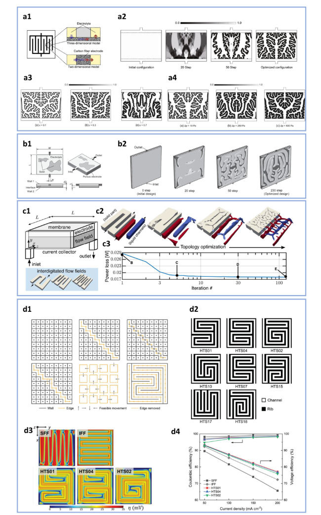
Fig. 11 a1 Comparison of flow field with respect to two- and three-dimensional analysis models in the case of an interdigitated flow field. a2 Optimization history of flow field configurations. Optimization configurations for different (a3) porosity settings and (a4) pressure drop settings (reproduced with permission from Ref. [37]). b1 Schematic of computational domain and boundary conditions. b2 Iteration history of topology-optimized flow fields (reproduced with permission from Ref. [88]). c1 Schematic of the half-cell computational domain. c2 Various design iterations during the optimization process. c3 The corresponding power loss during the optimization process (reproduced with permission from Ref. [89]). d1 Schematic of the key steps of the path generation algorithm. d2 Images of the eight promising flow fields selected from the screening process. d3 Simulated overpotential within the porous electrode. d4 CE and VE of the VRFBs with different flow fields (reproduced with permission from Ref. [38]) |
Based on the aforementioned studies, topology optimization provides a potential design pathway for generating irregular configurations by combining them with numerical models. The selection of initial patterns and maximized/minimized indicators significantly affects the final optimized configuration. It might be reasonable to use the total power loss or VEpump as the objective indicator for striking the balance between the electrochemical and hydraulic performance. However, it is worth noting that the irregular structure is hard to process with conventional fabrication approaches, and 3D printing technology may facilitate the application of topology optimization to the flow field design in RFBs. In addition, the topology optimization is currently applied to lab-scale flow fields. When applying topology optimization to stack-scale cells, there will be a significant increase in computational cost, which can be mitigated by using simplified numerical modeling and considering geometry similarity. Besides, the effect of optimization method still needs to be validated experimentally in the scale-up of RFBs.
Different from the iterative optimization of flow field configuration, Wan et al. constructed a flow field library, predicted the performance with machine learning and selected structures with high performance. Specifically, the first procedure was to generate a large amount of flow field designs. The active area as well as channel to rib ratio were fixed, and the inlet and outlet were connected to avoid excessive variety of configurations. As shown in Fig. 11d1, the active area is divided into several blocks. The initial flow channel region is represented in yellow. The random movement of the flow channel was then set until the channel to rib ratio attains 0.5 and a total of 11,564 configurations were generated. Next, 1164 flow fields were imported into the three-dimensional numerical model to obtain the reactants distribution and pressure drop. The relationship between the performance and 1164 flow field patterns were then extracted to train the convolutional neural network (CNN), based on which the performance of all the generated configurations were predicted with a low resource cost. In the end, eight configurations with a uniform reactant distribution and low pressure drop were determined and validated with both experiments and numerical simulation, as depicted in Fig. 11d2-d4. It should be noted that the flow channel arrangement of the eight configurations is similar to the reported convection-enhanced flow field in Fig. 9c [38]. The rotary channels induce a larger pressure difference between the adjacent flow channels, thereby enhancing the under-rib convection and battery performance. To sum up, the machine learning-assisted design pathway performs well in high-throughput screening of configurations due to the high accuracy and low resource cost. The advantages also make it promising in optimizing the geometric parameters and designing the configurations with unconnected inlet/outlet (such as interdigitated flow field). The design principles also apply to stack-scale batteries. With an enlarged active area, there will be more patterns in the flow field library, which increases the cost of dataset construction and neural network training. Moreover, as the channel length increases and the patterns become more complex, there might exist more promising flow fields that cannot be generated at small-scale sizes.
4 Flow field structure optimization
In addition to proposing novel flow field configurations, optimizing the geometric parameters and modifying the flow channels of flow fields are also of great significance in improving the battery performance. Generally, the flow fields have channels and ribs with the same width, and the geometric dimensions are determined intuitionally. However, as the battery scales and assembling conditions vary, it is necessary to tailor the key geometric parameters for striking the balance between electrochemical polarizations and pumping loss. In this section, the parametric investigation based on conventional serpentine and interdigitated flow fields is firstly presented, which provides guidance for applying the flow fields to high-performing RFBs. Moreover, considering that the currently adopted flow channels have a rectangular cross section and are caved on the surface of graphite plate, extensive research work has been carried out to optimize the flow field by modifying the cross section of flow channels and engraving the flow fields on electrodes, which enables an enhanced under-rib convection and alleviates the pressure drop. The detailed implementation methods, such as introducing the obstructions and ramps, as well as the influence on the battery performance will be thoroughly discussed, as shown in Fig. 12.
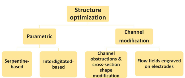
Fig. 12 Outlines for structure optimization of flow fields |
4.1 Parametric optimization
Geometric parameters of flow fields play a crucial role in deciding the battery performance by directly influencing the mass transport process and flow resistance. It is worth noting that adjusting the parameters usually affects the electrochemical performance and hydraulic performance inversely. To be specific, a small channel to rib ratio results in more uniform electrolyte distribution for both serpentine and interdigitated flow fields, which, however, leads to significantly increased pumping loss. Therefore, optimizing the geometric dimensions based on overall SE is essential for obtaining the optimal combination of parameters. In this section, we will discuss the influence of typical parameters, such as channel width, land width and channel depth, in serpentine and interdigitated flow fields, respectively. Parametric optimization under varying operating conditions and electrode properties will also be included.
For the conventional serpentine flow fields, the investigation objects usually include the channel size and channel to rib ratio under a given active area. Decreasing the channel width and channel to rib ratio can both diminish the mass transport polarization while increase the pumping power loss [40,90,91]. For example, Lee et al. investigated the effect of channel size on electrochemical reactions and fluid dynamics under a wide range of flow rates with a three-dimensional model. The channel width ranges from 1.9 mm to 9.6 mm, as shown in Fig. 13a1. It is found that there is a diminishing return on reducing the mass transport overpotential by decreasing the channel size and increasing the flow rate, as depicted in Fig. 13a2. As a result, the maximum power-based efficiency of 96.6% in Fig. 13a3 is obtained with the channel size of 1.9 mm at 60 mL min−1 [40]. Gundlapalli et al. revealed that widening channels can reduce the pressure drop without negatively impairing electrochemical performance. However, the electrode intrusion into channels is inevitable with wide channels adopted, as shown in Fig. 13b, which adversely affects both the pressure drop and electrochemical reactions [90].
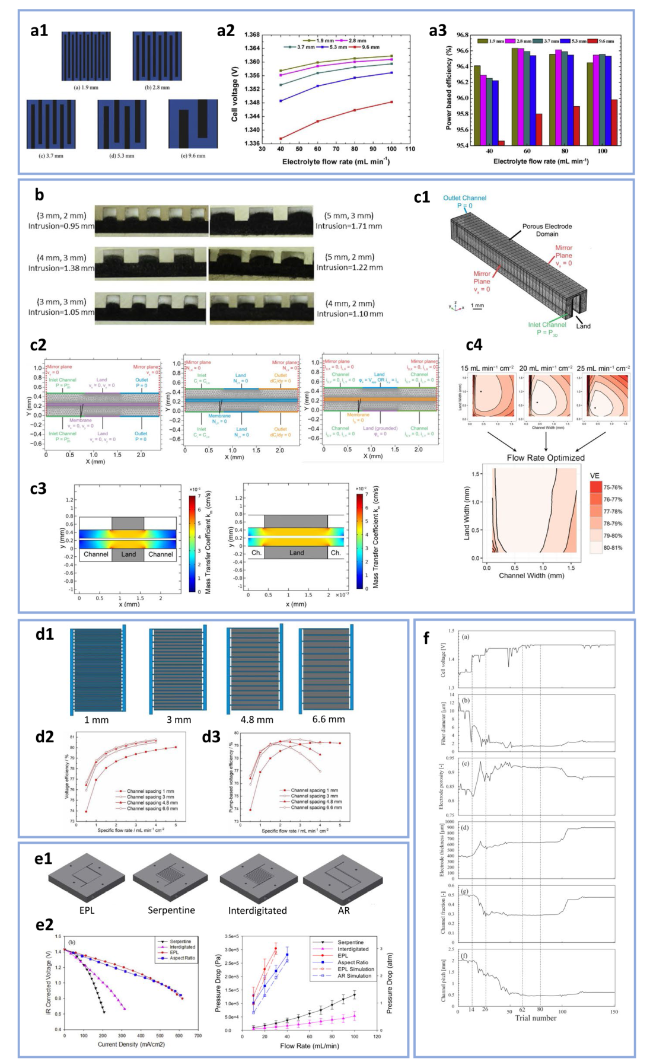
Fig. 13 a1 Schematics of five different serpentine flow fields. a2 Calculated cell voltage against the electrolyte flow rate and channel size. a3 Power-based efficiency according to the various flow rates and channel sizes (reproduced with permission from Ref. [40]). b Visualization of electrode intrusion into flow channels (reproduced with permission from Ref. [90]). c1 Boundary conditions for the three-dimensional fluid dynamics model. c2 Boundary conditions for the two-dimensional model coupling the fluid flow, mass transfer and electrochemical reactions. c3 Color map of the mass transfer coefficient in the “wide channel” (left) flow plate and “wide land” (right) flow plate. c4 Illustration of optimization on flow rate. The results from computations at various flow rates are combined to produce a single map of VEpump optimized with respect to flow rate (reproduced with permission from Ref. [92]). d1 The computational domain of interdigitated flow fields with different channel spacings. d2 VE and d3 VEpump of different channel spacings at a discharge current density of 200 mA cm−2 (reproduced with permission from Ref. [93]). e1 Flow field designs of Equal Path Length (EPL), Serpentine, Interdigitated and Aspect Ratio (AR) patterns. e2 Polarization curves and pressure drops of cells with different flow plates (reproduced with permission from Ref. [30]). f Values of various parameters and cell voltage during the multiple-parameter optimization process (reproduced with permission from Ref. [66]) |
Additionally, the effect of the interdigitated channel and rib dimensions on battery performance has also been studied. Considering that the flow behavior from each inflow branch channel into adjacent outflow branch channels is similar, the computational domain of interdigitated flow field is usually simplified to include only two channels and electrodes, as introduced in Section 2. As shown in Fig. 13c1, Gerhardt et al. constructed the three-dimensional fluid dynamics model, including a half inflow channel and a half outflow channel. Then, the authors further developed a two-dimensional model to interpret the electrochemical reactions, in which the inlet pressure is applied to the interface between the inflow channel and electrodes, as depicted in Fig. 13c2. The color map of mass transfer coefficient in Fig. 13c3 shows that the stagnant fluid zones above central lines of the interdigitated channels negatively affect the cell performance. By combining the pumping power in three-dimensional model and polarization results in two-dimensional model, the flow fields with different channel and rib widths were compared based on VEpump. Since the flow rate is an easily adjustable parameter in practice, all the flow fields are assumed to operate with respective most efficient flow rates and VEpump with different flow rates are combined into one single graph, as shown in Fig. 13c4. It is found that the optimal channel width does not change, but a wide range of rib widths becomes accessible because the flow rate can be adjusted to accommodate varying rib widths [92].
Li et al. analyzed the effect of spacing between adjacent channels with a fixed active area. As shown in Fig. 13d, it is revealed that VEpump shows a first increase and then decreases as the specific flow rate increases. This is because the pumping loss plays a more dominant role in influencing the overall performance at large flow rates. The maximized VEpump of 79.1% is reached with the optimal channel spacing of 3 mm at 200 mA cm−2 and 4.5 mL min−1 cm−2 [93]. You et al. optimized the number and size of channels to strike the balance between the pressure drop and electrolyte distribution in the electrode, which affects the pumping consumption and mass transport, respectively. Increasing the channel depth and width is effective to lower the pressure drop and enhance the distribution uniformity of electrolyte [45]. Prumbohm et al. also declared that a large channel height and width as well as small land width lead to a low pressure drop with a cell-level three-dimensional model. As for the electrochemical performance, improving the limiting current density depends primarily on increasing the land width. Nevertheless, there still exits a diminishing return on reducing the polarizations by continuously expanding the land width [94].
Guo et al. demonstrated that in addition to the stagnant zone above the channel, the electrolyte distribution along the branch channels also significantly impacts the battery performance. Key geometric parameters including the unit aspect ratio and channel fraction were systematically investigated with a three-dimensional model. Results show that large aspect ratios and small channel fractions reduce the mass transport loss by diminishing the stagnant zone in the under-channel region. However, when the aspect ratio exceeds a critical value, the extremely long and narrow flow field results in an uneven distribution of reactants along the channel, thereby increasing the polarization greatly. Moreover, the simulation was then applied to a larger active area for identifying the design pathway in the scale-up. It is shown that larger aspect ratios are beneficial to alleviate the dramatically increased pressure drop [62]. Houser et al. studied the effect of active area shape with flow-through configuration and compared it with serpentine and interdigitated flow fields. As shown in Fig. 13e, among the four flow plates, the equal path length (EPL) and aspect ratio (AR) structures deliver larger limiting current densities, but much higher pressure drops compared to the serpentine and interdigitated flow fields. Notably, the adoption of AR structure rather than EPL structure leads to lower pressure drop due to the shorter convection path [30].
Considering that the optimal flow field geometry may vary with the electrodes and assembling conditions, Tsushima et al. supplemented the investigation of electrode properties (including fiber diameter, porosity, and electrode thickness) with a two-dimensional model and conducted the multi-parameter optimization. The cell voltage is ultimately improved from initial 1.351 V to 1.450 V after 80 iterations, as shown in Fig. 13f [66].
As summarized above, when improving the SE through parametric optimization, the parasitic effect such as electrode deformation may also negatively affect the battery performance. Therefore, the category and scope of optimized parameters should be carefully determined. On this basis, multi-parameter optimization is essential in engineering applications especially for stack-scale batteries, since the optimal values may vary as the other geometric parameters and assembling conditions change. The simplified modeling and optimization algorithms are expected to accelerate the optimizing process.
4.2 Structure modification
4.2.1 Modification in flow channels
Modification in serpentine flow field As introduced in Section 3.1, the serpentine and interdigitated flow fields are the most widely researched configurations. However, dead zones still exist with weak convection of electrolytes in the two patterns, which leads to nonuniform distribution of electrolytes. In this section, we will summarize strategies by modifying the channels to enhance the distribution uniformity in serpentine and interdigitated flow fields. Typically, blocks, obstructions, or pillars are introduced to enhance the electrolyte penetration into the electrodes. The designs of such blocks differ for the serpentine and interdigitated patterns due to the different characteristics of the two structures.
For the serpentine flow field, the pattern is repeated by U-shaped segment, and the connected end leads to a lower pressure difference between the neighboring channels while the other end exhibits higher, such variation leads to the nonuniform electrolyte distribution in the electrodes, as shown in Fig. 9b. Accordingly, Lu et al. placed blocks with different heights at the turning short channels to intensify the under-rib convection, which inevitably leads to increased pressure drop. As optimized by the author with a three-dimensional model, the block with a height of 1.4 mm leads to the highest SE [95] (Fig. 14a). Differently, Pan et al. modified the channel depth along the whole flow path to improve electrochemical performance. This is because although all the ribs have a similar velocity distribution, the downstream electrolyte lacks reactants due to the continuous consumption of electrochemical reactions, thereby inducing an uneven reactants distribution over the entire electrode. Therefore, the channel depth is linearly reduced from the inlet and outlet for speeding up the electrolyte velocity and enhancing the convection near the outlet, which leads to an increase in EE by 5% at 12 mL min−1 cm−2 and 400 mA cm−2 [96].
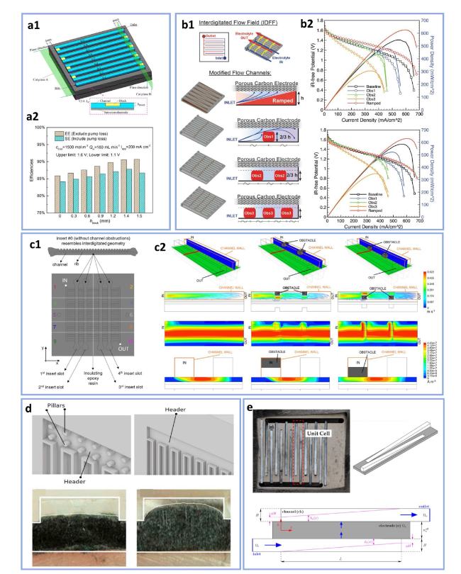
Fig. 14 Modification in flow channels. a1, a2 Serpentine flow channels modified with obstructions (reproduced with permission from Ref. [95]), b1, b2 interdigitated flow channels modified with ramps and obstructions (reproduced with permission from Ref. [97]), c1, c2 influence of locations and numbers of obstructions in interdigitated flow channels (reproduced with permission from Ref. [39]), d channels with pillars to avoid electrode intrusions (reproduced with permission from Ref. [98]). e tapered channel design for interdigitated flow field (reproduced with permission from Ref. [99]) |
Modification in interdigitated flow field Akuzum et al. investigated the effects of varying channel depths using ramps or obstructions on both the electrochemical performance and pressure drop in the interdigitated flow field, as shown in Fig. 14b. Four different channel configurations were investigated, including a ramped channel and channels with varying numbers of obstructions. It was found that ramped channel leads to an improved electrochemical performance by increasing the electrolyte penetration depth in the electrode, especially on the electrode-membrane interface. However, adding obstructions in the channel leads to even worse electrochemical performance, which is possible due to the “by-pass” of electrolyte that the electrolyte travels to the outlet after encountering the obstructions. In addition, it is interesting to find that the tapered channel and channels with obstructions lead to an even smaller pressure drop compared with the flow field without any modifications. These conclusions of adding obstructions in interdigitated flow channels differ from that in the serpentine flow field, which may come from the different flow paths in the two distinct geometries [97].
A systematic study of the location of the obstructions and their effectiveness in improving the cell performance in interdigitated flow fields is carried out by Messaggi et al. Specifically, two types of obstructions located on the channel wall or the electrode interface were investigated, as shown in Fig. 14c. As revealed from the simulation, obstructions on the channel side contribute to the electrolyte penetration into the porous electrode, while obstruction on the electrode interface allows part of the electrolyte to reach the channel end. Therefore, the channel side obstruction is more effective to be placed close to the electrolyte outlet to compensate for the consumption of the reactants. Obstructions at the electrode interface are more effective to be placed close to the electrolyte inlet and induce higher under-rib convection, which leads to higher overall performance [39].
Typically, pillars, obstructions, or blocks are placed in the channels to enhance the electrolyte convection into the electrodes. In addition to such functions, the pillars can work as supports for electrodes under compression, reducing the electrode intrusion into channels. Actually, the issues of electrode intrusion into channels become even more severe when the flow field scales up, which may lead to dramatically increased flow resistance and uneven electrolyte distribution. As reported by Gundlapalli et al., pillars were placed in the manifold of the interdigitated flow field to mitigate the electrode intrusion in the 900 cm2 and 1500 cm2 cells [98] (Fig. 14d).
In addition to placing obstacles in the channels to increase the electrolyte velocity, adjusting the geometry of the channel cross-section can also enhance the electrolyte velocity. However, the enhancement in reactant transport versus the increase in the pumping loss should be discussed. García-Salaberri et al. modeled the effect of channel tapering on the pressure drop and flow distribution, as shown in Fig. 14e. Since the pressure drop in the interdigitated flow fields comes from both the channel and the electrodes, the increase in pressure drop in tapered channels is tightly related to the electrode properties. Such effect was also discussed in García-Salaberri et al.’s findings. For electrodes with high permeability, pressure drop in channels accounts for the total pressure drop. Therefore, the pressure drop in the cells with tapered flow channels would be much higher than that in the constant cross-section flow channels, and the enhancement in the electrochemical performance may not compensate for the increased pumping consumption. However, for electrodes with low permeability, tapered flow fields can lead to a higher SE with a similar pumping loss [99].
Other modifications in the channels include changing the shapes of the cross-section, e.g., triangular, semi-circle or trapezoidal channels [100]. Either adding obstructions or changing the shapes of the channel cross-section is aimed to enhance the electrolyte penetration into the electrode. However, the parasitic influence on the pressure drop should be considered together with the electrochemical performance. In addition, the results may vary for different flow patterns, operating conditions, and cell scales. Currently, it is difficult to reach a consensus for optimizing channel modification, and more systematic research work involving both experimental and numerical strategies is expected to give more fundamental insights. Furthermore, in addition to the tradeoff between possibly increased pressure drop and electrochemical performance gains, manufacturing and assembly issues must be taken into account when modifying channels during scale-up. These considerations may be combined with parametric optimization for flow field scale-up.
4.2.2 Flow fields engraved on electrodes
Even though the flow-by cell architecture leads to both improved electrochemical performance and a lower pressure drop, the high manufacturing cost and sealing pressure hinder the scale-up of flow fields. In this regard, some researchers proposed engraving channels in electrodes to distribute electrolytes instead of flow channels. There are mainly three different types of engraving channels on electrodes. The first type is engraving channels through the whole thickness of the electrode. Yin et al. studied electrodes engraved with interdigitated flow fields using a 3D numerical model and compared it with flow fields in graphite plate and flow-through configurations, as shown in Fig. 15a. It is simulated that the electrodes cut with flow field exhibit the lowest pressure drop. Even though the cell with engraved electrodes shows slightly lower SE than the flow-through configurations at a low flow rate (1 mL min−1), it performs much better at increased flow rates. Actually, there exists an optimal flow rate to reach the highest SE for a particular cell configuration, and the optimal flow rate differs for different flow field structures [101].
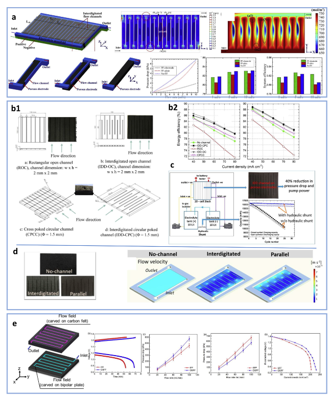
Fig. 15 Flow fields engraved on electrodes. a Numerical analysis of engraving electrodes with cut-through interdigitated channels (reproduced with permission from Ref. [101]), b1, b2 engraving electrodes with a certain depth of different channel patterns (reproduced with permission from Ref. [102]), c electrodes with flow channels for scaled-up cells (reproduced with permission from Ref. [103]). d other patterns of flow channels engraved on electrodes (reproduced with permission from Ref. [104]), and e detached electrode-flow field design (reproduced with permission from Ref. [105]) |
Cutting channels over the whole thickness of the electrode may lead to difficulties in assembling the electrodes in the cells since the electrodes are composed of separating pieces. Therefore, the second type of engraving channels on electrodes is to cut a certain depth in the channel while the electrode can keep its integral structure. Bhattarai et al. experimentally investigated four types of electrodes with channels, which were rectangular open channel, interdigitated open cut channel, interdigitated circular poked channel and cross poked circular channels in cells with an active area of 100 cm2, as shown in Fig. 15b. For the first two types, channels were made on the surface of electrodes, while the latter two constructed channels inside the electrode. Results show that engraving interdigitated type channels, including on the electrode surface and bedding inside electrode, can lead to improved cell performance, while the former mainly reduces the pressure drop and the latter mainly improves the electrolyte distribution uniformity [102]. The same group later scaled up the electrodes with interdigitated flow channels to a 20-cell 1 kW VRFB stack, which demonstrates stable performance in achieving an EE of 80.5% at 80 mA cm−2, showing the potential for electrodes with channels to be scaled-up [103] (Fig. 15c). Hao et al. constructed some parallel channels with different lengths and one open end on the electrode, which demonstrates higher performance than electrodes with interdigitated channels (Fig. 15d) [104].
The third type of engraving channels on the electrode is to cut part of the channels on the graphite plate and part of the channels on the electrodes. As reported by Sun et al., staggered serpentine channels were constructed on the plate and electrode (near membrane side), which enhance the mass transport in both the in-plane and through-plane directions, as shown in Fig. 15e [105]. Compared with the conventional interdigitated flow field, the detached serpentine configuration leads to improved mass transport, though slightly increased pressure drop. Therefore, a 3.2% increase in SE (v.s. interdigitated flow field) is achieved at a current density of 100 mA cm−2, an electrolyte flow rate of 20 mL min−1, and a compression ratio of 40%. Compared with the serpentine flow field, the detached serpentine configuration leads to lower pressure drop and enhanced electrolyte mass transport.
As summarized above, all three types of constructing channels in the electrodes are effective in reducing the pressure drop and improving the electrolyte distribution uniformity. Considering the construction feasibility and effectiveness, the second type of engraving open channels on electrodes seems more applicable in practical applications, especially for scaled-up stacks.
5 Flow field scale-up
When scaling up the RFBs, the pressure drop increases sharply, which necessitates a relatively low flow rate to accommodate the pumping work. However, the lower flow rate and longer flow path would exacerbate the distribution non-uniformity of electrolytes. As introduced in Section 3.1, the rules of the pressure drop and electrolyte distribution for different flow fields are quite different. When the flow fields are scaled up, the response of the pressure drop and electrolyte distribution also differs. For a single serpentine flow field, the increased flow distance passing through the whole active area domain would lead to a dramatically increased pressure drop. In addition, the pumping work is exponentially increased with the flow rate, as simulated in Ref. [23] with an active area of 410 cm2 (Fig. 16a). In the meantime, the electrolyte distribution along the flow path would become more nonuniform. Splitting single serpentine channels into several parallel serpentine channels reduces the flow flux and distance in each separate serpentine channel, thus reducing the total pressure drop. However, the electrolyte distribution may be deteriorated with the increased number of flow channels since the weak under-rib convection between parallel channels may lead to zones with poor mass transport. In addition to splitting the single serpentine flow field into parallel serpentine channels, Kumar et al. split the serpentine channel over the active area of 100 and 414 cm2, respectively [106] (Fig. 16b). Such scale-up methods lead to decreased pressure drop but may also lead to poor electrochemical performance. Therefore, the SE, including the pumping work, should be considered to evaluate the scaled-up patterns.
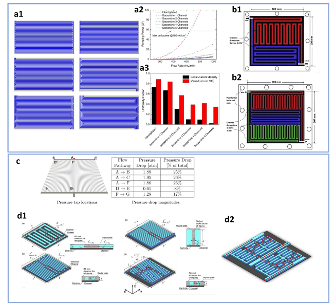
Fig. 16 Scaled-up strategies for serpentine- and interdigitated-based flow fields. a1, a2 Parallel splitting strategy for serpentine flow field (reproduced with permission from Ref. [23]), b1, b2 splitting serpentine flow field based on separate areas (reproduced with permission from Ref. [106]), c pressure distribution in interdigitated flow field (reproduced with permission from Ref. [46]), d1, d2 different pathways to scale-up flow fields (reproduced with permission from Ref. [32]) |
For the interdigitated flow field, the pressure drop also scales with the active area. In addition, according to the simulation by Knudsen et al. (Fig. 16c) [46], the pressure drop inside the manifold accounts for a large proportion when the active area scales to 400 cm2. Therefore, the geometric parameters of the flow field should be optimized to lower the pressure drop. Meanwhile, the non-uniformity among different branch channels and along the branch channel becomes even more severe at enlarged scales. In some studies, constructing hierarchical channels is found to decrease the pressure drop by splitting the electrolyte, as introduced in Section 3.2.1, which makes the novel structures applicable in scaled-up flow cells to alleviate the large pumping loss. For example, Zeng et al. designed a hierarchical interdigitated flow field by introducing the secondary branch channels connected to the primary branch channels. The cross-sectional area is gradually decreased from the main channel to the primary and secondary branch channels. At a flow rate of 3 mL min−1 cm−2, the pumping loss is decreased by 65.9%, and the VEpump increases from 73.8% to 79.1% at 240 mA cm−2 [18]. Guo et al. retained the conventional interdigitated channels in the active area but designed bifurcate distribution/collection channels outside the active area, which can split the electrolyte evenly and lower the pressure drop simultaneously [84]. Gundlapalli et al. scaled the interdigitated flow field by extending the pins along the inlet branch channels [107]. Guo et al. investigated geometric parameters (aspect ratio, channel fraction, channel depth) of a unit interdigitated flow field, and scaled the area of the unit from 60 to 540 mm2, the latter of which corresponds to an active area of 345.6 cm2 with 32 units. It is found that the effect of pumping loss on VEpump becomes more significant during scale-up, hence a larger aspect ratio (channel length to width) is preferred to lower the flow resistance in the electrodes for the scaled unit. In addition, the optimal flow rate decreases after the enlargement due to the intensified pumping loss [62].
Sun and Zheng et al. proposed different pathways to enlarge the interdigitated flow fields on an active area of 900 cm2, which are geometric similarity, channel length extension, same pressure drop, and split-interdigitated flow field (Fig. 16d). In the geometric similarity strategy, the channel number and height keep the same, while the width and length of the channel increase by the scaling-up factor. Compared with small-scale battery performance, the geometric similarity scale-up leads to a ~ 10 times increase in pressure drop, while the increased flow distance intensifies the distribution non-uniformity, which leads to a ~ 4% drop in the overall EE. The “channel length extension” strategy keeps the cross-sectional area of the channel unchanged by increasing the number and length of channels, leading to extremely uneven distribution of electrolytes and increased pressure drop, contributing to ~ 2.6% drop in the overall EE. The “same pressure drop” strategy enlarges the cross-sectional area of channels, which leads to manufacturing toughness and high concentration overpotential, and ~ 5.2% loss in overall VE. The “split interdigitated flow field” leads to an even distribution of electrolytes over the active area and a close performance to small cells. Although factors such as operating conditions and electrode/electrolyte properties influence the results, splitting the interdigitated flow field and widening the channel width are promising strategies to reduce the pressure drop after scale-up [32]. In addition, as shown in Fig. 16d2, widening the main channels can decrease the pressure drop while having little effect on the electrochemical performance of the battery.
In addition, the scale-up of flow-through configuration also leads to quadratically increased pressure drop and electrolyte maldistribution. Constructing inlet and outlet distribution channels leads to a more uniform electrolyte distribution in the electrode. Moreover, constructing channels on the electrode is proven effective in better distributing electrolytes [103]. In summary, there are different pathways to scale up the flow field to alleviate pressure drop and distribute electrolytes. Even though the geometric parameters for serpentine and interdigitated flow fields are different, splitting the two flow channels and adjusting the geometric parameters are effective in reducing the pumping work in the scaled-up applications. In addition to increased pressure drop and nonuniform distribution during the scale-up process, other issues related to the manufacturing and assembly should also be considered, e.g., the electrode intrusion in channels could be severe if the channel width or depth is not scaled reasonably [90,106].
6 Concluding remarks and perspectives
RFBs are promising techniques for large-scale energy storage and have surging commercial demands due to their easy scalability, site independence, and high safety. With the increasing demand for storing the electricity generated by renewable energies, there have been a growing number of commercial demonstrations of VRFBs. Even though relatively high operating current and power densities are achieved in lab-scale RFBs [28,108], such performance is hard to be duplicated in scale-up cells. The limiting factors are the dramatically increased pumping power and intensified electrolyte distribution non-uniformity. Therefore, the cell configuration and flow field design become particularly essential for developing next-generation RFBs, and this review summarizes the recent advances in flow pattern design, structure optimization, and the key issues during the scale-up process.
We first overviewed the strategies, including numerical and experimental, in evaluating the transport properties and electrochemical performance of RFBs with different flow patterns. Typically, experimental methods such as battery or hydraulic tests directly compare the cell performance, which, however, can only give case-by-case information and could be quite time-consuming and cost-ineffective. Diverse numerical simulation methods have emerged as indispensable tools for multi-parameter and multi-object optimization. The scale, complexity, accuracy, cost, and revealed information differ among simulation methods. In some cases, more than one simulation strategy is combined to better uncover and interpret the experimental results.
Then, we comprehensively discussed the electrolyte transport of flow-through and flow-by structures. Among numerous classic flow field patterns, we elaborated on comparing serpentine and interdigitated flow fields. Typically, the flow-field-structured configuration leads to a lower pressure drop and better electrochemical performance than the flow-through configuration. However, results could vary when comparing flow patterns under different assembling and operating conditions. Therefore, the electrode properties, compression ratio, flow rate, and operating current should be paired with the flow field optimization. Moreover, we summarized the novel pattern designs from intuition-based as well as topology- and machine learning-assisted methods, which provide new guidelines and possibilities for pattern design in the future.
As an important part of this review, the structure optimization of different flow fields is thoroughly discussed from geometric parameters and channel modification aspects. It is worth pointing out that an optimal combination of geometric parameters obtained by multi-parameter optimization algorithm is critical for practical applications. In addition, modifications in channels, such as placing obstructions in channels or varying the shape of the cross-section are common strategies to enhance electrolyte convection. However, when we evaluate the performance of flow fields, the operating conditions and electrode properties should be well considered since the electrolyte transport and electrochemical reaction is an overall effect of all the components and operating conditions.
At the current stage, constructing high-performance flow configurations becomes urgent for the scale-up of RFBs. Therefore, we extensively reviewed the issues and strategies in the scale-up process. The dramatically increased pumping work and non-uniformity are the two main challenges for performance enhancement in scaled-up RFBs, and there are different pathways to scale flow fields. It seems that splitting the flow fields combined with parametric optimization is effective in reducing the pressure drop and increasing distribution uniformity for the serpentine and interdigitated patterns. In the future, numerical modeling is expected to assist flow pattern optimization and provide scale-up pathways for practical applications. In addition, the scaling of flow-field-structured configuration on a graphite plate would highly increase the capital cost of a battery stack. Therefore, engraving flow patterns on electrodes for the flow-through structure is another potential strategy for scaled-up battery design.
In summary, the serpentine and interdigitated flow fields are still the most popular patterns for RFBs. And these two patterns show distinct features and respond differently to the assembling and operating conditions. Till now, most pattern designs, parametric optimization, and scale-up designs are developed based on the two types of flow patterns. Multi-parameter optimization has also been utilized to obtain the optimal combination of key geometric dimensions and assembly parameters for maximizing the electrolyte distribution uniformity at a minimized pressure drop. In addition, topology optimization and machine learning offer more possibilities for novel pattern design and screening. It is expected that the collaborative design process combining the numerical simulation, structural optimization and experimental tests will promote the development of cell configuration design for practical RFBs applications.
Abbreviations
RFB $\ \ \ \ \ \ \ \ $Redox flow battery
ARFB $\ \ \ \ \ \ \ \ $Aqueous redox flow battery
VRFB $\ \ \ \ \ \ \ \ $Vanadium redox flow battery
EE $\ \ \ \ \ \ \ \ $Energy efficiency
EU $\ \ \ \ \ \ \ \ $Electrolyte utilization
SE $\ \ \ \ \ \ \ \ $System efficiency
CE $\ \ \ \ \ \ \ \ $Coulombic efficiency
VE $\ \ \ \ \ \ \ \ $Voltage efficiency
CFD $\ \ \ \ \ \ \ \ $Computational fluid dynamics
FEM $\ \ \ \ \ \ \ \ $Finite element method
CNN $\ \ \ \ \ \ \ \ $Convolutional neural network
EPL $\ \ \ \ \ \ \ \ $Equal path length
AR $\ \ \ \ \ \ \ \ $Aspect ratio
Acknowledgements
Not applicable.
Authors’ contributions
JS and ZG organized the outline of the manuscript, drafted, and revised the manuscript. LP, XF, and LW commented on the previous versions of the manuscript and revised the manuscript. TZ conceptualized the manuscript and revised the manuscript. We ensure that all authors are included in the author list and its order has been agreed by all authors. All authors read and approved the final manuscript.
Funding
Open access funding provided by Shanghai Jiao Tong University. This work was supported by the National Natural Science Foundation of China (No. 52206089), Joint Research Center on Energy Storage Technology in Salt Caverns Program (TO2203001), and Research Grants Council of the Hong Kong Special Administrative Region, China (Project No. T23-601/17-R).
Availability of data and materials
The data and material are available upon request.
Declarations
Ethics approval and consent to participate
Not applicable.
Consent for publication
Not applicable.
Competing interests
Prof. Tianshou Zhao is an editorial advisory board member for Carbon Neutrality and was not involved in the editorial review, or the decision to publish this article. All authors declare that there are no competing interests.
Publisher’s Note
Springer Nature remains neutral with regard to jurisdictional claims in published maps and institutional affiliations.
