Applications of cnoidal and snoidal wave solutions via optimal system of subalgebras for a generalized extended (2+1)-D quantum Zakharov-Kuznetsov equation with power-law nonlinearity in oceanography and ocean engineering

Oke Davies Adeyemo

doi:10.1016/j.joes.2022.04.012

Journal of Ocean Engineering and Science >

2024 , Vol. 9 >Issue 2: 126 - 153

DOI: https://doi.org/10.1016/j.joes.2022.04.012

Research article

Applications of cnoidal and snoidal wave solutions via optimal system of subalgebras for a generalized extended (2+1)-D quantum Zakharov-Kuznetsov equation with power-law nonlinearity in oceanography and ocean engineering

Oke Davies Adeyemo

Expand

International Institute for Symmetry Analysis and Mathematical Modelling, Department of Mathematical Sciences, North-West University, Mafikeng Campus, Private Bag X 2046, Mmabatho 2735, Republic of South Africa

E-mail address: 29532892@student.g.nwu.ac.za

Received date: 2022-03-09

Revised date: 2022-04-14

Accepted date: 2022-04-18

Online published: 2022-04-26

Fold

Abstract

The nonlinear evolution equations have a wide range of applications, more precisely in physics, biology, chemistry and engineering fields. This domain serves as a point of interest to a large extent in the world's mathematical community. Thus, this paper purveys an analytical study of a generalized extended (2+1)-dimensional quantum Zakharov-Kuznetsov equation with power-law nonlinearity in oceanography and ocean engineering. The Lie group theory of differential equations is utilized to compute an optimal system of one dimension for the Lie algebra of the model. We further reduce the equation using the subalgebras obtained. Besides, more general solutions of the underlying equation are secured for some special cases of n with the use of extended Jacobi function expansion technique. Consequently, we secure new bounded and unbounded solutions of interest for the equation in various solitonic structures including bright, dark, periodic (cnoidal and snoidal), compact-type as well as singular solitons. The applications of cnoidal and snoidal waves of the model in oceanography and ocean engineering for the first time, are outlined with suitable diagrams. This can be of interest to oceanographers and ocean engineers for future analysis. Furthermore, to visualize the dynamics of the results found, we present the graphic display of each of the solutions. Conclusively, we construct conservation laws of the understudy equation via the application of Noether's theorem.

Highlights

● We study cnoidal and snoidal wave solutions via optimal system of one-dimensional sub-algebras for a generalized extended (2+1)-D quantum ZK equation with power-law non-linearity in oceanography and ocean engineering.

● We obtain non-topological soliton, cnoidal and snoidal wave and hyperbolic solutions.

● We derive conservation laws using Noether's theorem.

● We highlight the applications of our results (cnoidal and snoidal waves) in oceanography and ocean engineering.

Key words： A generalized extended (2+1)-dimensional quantum Zakharov-Kuznetsov equation; Lie point symmetries; Optimal system of subalgebras; Cnoidal and snoidal waves; Extended Jacobi function expansion technique; Conservation laws

Cite this article

Oke Davies Adeyemo . Applications of cnoidal and snoidal wave solutions via optimal system of subalgebras for a generalized extended (2+1)-D quantum Zakharov-Kuznetsov equation with power-law nonlinearity in oceanography and ocean engineering[J]. Journal of Ocean Engineering and Science, 2024 , 9(2) : 126 -153 . DOI: 10.1016/j.joes.2022.04.012

1. Introduction

The nonlinear evolution equations, as well as their solutions, are highly significant with regards to a good understanding of diverse physical phenomena, for example, in the investigation of the waves observed in plasma, astrophysics, optical fibers, laser, fluids, water waves alongside other areas bothering on engineering. Investigation of autonomous nonlinear evolution equations possesses largely a very rich and long history. For instance, in [1], the generalized variable coefficient Korteweg-de Vries equation with dual power-law nonlinearities possessive of linear damping as well as dispersion terms in quantum field theory were studied. Besides, the significance of the equation in quantum field theory and other theoretic physics areas were highlighted. Moreover, a generalized system of variable-coefficient modified Kadomtsev-Petviashvili-Burgers-type equation in three dimensions was examined in [2]. The authors in [3], investigated the generalized advection-diffusion equation, an important nonlinear evolution equation in fluid mechanics, featuring the transit of buoyancy-projecting-plume existing in a bent-on bibulous medium. A generalized Korteweg-de Vries-Zakharov-Kuznetsov equation in [4], was also examined. The equation recounts the fusion of warm inviscid fluid and hot isochoric alongside a cold static environment which has significance in fluid dynamics. Besides, in [5], a modified-generalized Zakharov-Kuznetsov (ZK) model, delineating ion-acoustic gravitation solitary waves found in a magnetoplasma-electron-positron-ion that exists in the primordial universe was contemplated. This equation was invoked in modelling situations in plasma physics. Moreover, in [6] a study was carried out on interaction characteristics of the vector bright solitons observed via the examination of the coupled Fokas-Lenells system. This system models the femtosecond optical pulses existing in a birefringent optical fibre.

Consequently, nonlinear evolution equations have continued to attract the attention of mathematicians and physicists in these recent years. Further to that, exact or analytic solutions to these equations have been regarded as the key tool for scientists to know the various physical happenstances that govern the real world today. Therefore, searching for exact travelling wave solutions relative to these nonlinear evolution equations plays a key role in the examination of nonlinear physical phenomena that can be associated with many other fields besides the aforementioned areas like meteorology, electromagnetic theory, nonlinear optics as well as other areas of science.

Meanwhile, in recent times scientists have developed effective techniques to obtain viable analytical solutions to nonlinear evolution equations, such as Cole-Hopf transformation approach [8], generalized unified technique [9], [10], exp

(- Φ (η))

-expansion technique[11], [12], F-expansion technique [1], Painlevé expansion approach [13], mapping technique and extended mapping technique [14], [15], Adomian decomposition approach[16], homotopy perturbation technique[17], Bäcklund transformation [18], rational expansion technique [19], tan-cot approach [20], extended simplest equation method[21], Hirota technique [22], Lie group analysis [23], [24], [25], [26], [27], bifurcation technique [28], the

(G^{'} / G) -

expansion method [29], Darboux transformation approach [30], sine-Gordon equation expansion technique [31], Kudryashov method [32], exponential function technique [33], [34], tanh-function technique[35], ansatz technique[36], [37], tanh-coth approach[38], and on and on, the list continues.

Many years back, Zakharov and Kuznetsov[39] introduced an equation modelling nonlinear ion-acoustic waves embedded in a magnetized plasma which comprises cold as well as hot isothermal electrons. The quantum plasmas alongside their new characteristics have captivated the attention of scientists from both theoretical as well as experimental standpoints. Due to the reason that it plays a key role in carrying charge whenever the de Broglie wavelength surpasses the Debye wavelength and as well as approaches the Fermi wavelength[40]. The character of the waves that are weakly nonlinear ion-acoustic which exists in the presence of a magnetic field that is described to be uniform, is administered by the quantum Zakharov-Kuznetsov (QZK) equation. Various authors have investigated the effect of such a magnetic field in diverse quantum plasma models [41].

The two-dimensional Zakharov-Kuznerov equation (ZK)[42]

(1.1)

u_{t} + u^{2} u_{x} + u_{x x x} + u_{x x y} = 0,

has been investigated by researchers. In [42], Krishnan and Biswas employed the mapping technique to achieve the solutions of (1.1). The solutions found include shock waves, cnoidal waves, and periodic singular waves alongside solitary waves. Besides, ZK Eq. (1.1) with power-law nonlinearity given as

(1.2)

q_{t} + a q^{n} q_{x} + b (q_{x x} + q_{x y})_{x} = 0,

was also studied by the authors where the ansatz approach was engaged in securing topological solitons and shock wave solutions for some specific values for the parameters of the power law. In [43], Abdou achieved the solutions of ZK (1.1) by utilizing the simplified form of Hirota's bilinear technique. Wazwaz [44], [45] studied equation (1.1) via the use of extended tanh, sine-cosine, with homotopy analysis techniques to gain solutions to the equation. He found solutions in the structure of soliton solutions. In addition, hyperbolic function solutions such as coth and tanh combined, new travelling wave solutions as well as periodic solutions were also gained. Moreover, the author in [46] obtained analytic solutions of the generalized version of (1.1) with time-dependent coefficients and nonlinear dispersion by employing the solitary wave ansatz technique. In [47], the authors found some closed-form solutions of (1.2) via Lie symmetry analysis. They also secure the conserved quantities of the equation by employing Ibragimov's conservation law theorem.

The new extended (2+1)-dimensional quantum Zakharov-Kuznerov equation (QZK) [48], [49]

(1.3)

u_{t} + a u u_{x} + b (u_{x x x} + u_{y y y}) + c (u_{x y y} + u_{x x y}) = 0,

with

a

b

and

c

regarded as real-valued constants whereas

u (x, y, t)

stands for electrostatic wave potential existing in plasmas which is obviously a function depending on spatial variables

x

y

as well as the temporal variable

t

. The first term in QZK (1.3) is regarded as the temporal term of evolution, the coefficient of

a

taken as the nonlinear term whereas the coefficient of

b

as well as that of

c

denotes the spatial dispersions which are multi-dimensional. The QZK equation (1.3) recounts ion-acoustic waves that are discovered to be included in a magnetized plasma consisting of hot isothermal alongside cold ions electrons. In [48], Wang et al. engaged group theorem to secure a plethora of analytic solutions of (1.3). Moreover, the authors in [49] found the closed-form solutions of QZK (1.3) with the use of a simplified structure of the bilinear technique, sech approach as well as tanh method. Multiple solitons solutions of the equation were gained. Lately, Jiang et al. in [50] carried out a Lie group analysis of the equation and achieved the conserved quantities of the equation via the utilization of Ibragimov's theorem for the conserved vector.

Remarkable is the fact that symmetry plays a highly significant role in various fields of nature, most especially in integrable systems for the existence of infinitely many symmetries. This technique was introduced towards the end of the nineteenth century, by the Norwegian mathematician, named Sophus Lie. The notion of the Lie group was to study the solutions to differential equations. Roughly speaking, one can say that a Lie point symmetry of a system refers to a local group of transformations that ensures the mapping of every solution of the system to another solution that belongs to the same system. The rigours of achieving an increasing number of solutions of systems of partial differential equations are associated with the group properties of these differential equations. In order to get the Lie point symmetry of a nonlinear equation, diverse effective methods have been proposed, such as the classical Lie group method[26], [51], nonclassical method [52], [53], symmetry reduction[54], [55], and so on. Lie's method is an efficient and the simplest technique among group theoretic techniques and a vast number of equations [56], [57] have been solved with the aid of this technique.

In the same vein, conservation laws have been viewed to serve a leading role in examining differential equations, since they delineate physical conserved quantities, consisting of energy, mass, momentum as well as charge together with other motion constants[4], [58]. Conservation laws have also been utilized to carry out investigations on the existence, uniqueness, as well as stability of solutions regarding nonlinear partial differential equations (NLNPDE) [59]. Moreover, they have as well been applied to numerical techniques [60]. In consequence, it is an optimum necessity to examine the conservation laws of partial differential equations.

1.1. Governing equation

In our study, we contemplate securing various solitary wave solutions of powerlaw nonlinearity [1], [3], [4] of a more generalized structure of (1.3) and it is called a generalized (2+1)-dimensional extended quantum Zakharov-Kuznetsov equation (3D-gextQZKe) given as

(1.4)

u_{t} + a u^{n} u_{x} + b u_{x x x} + c u_{y y y} + d u_{x y y} + e u_{x x y} = 0, a \neq b \neq c, b \neq e, d \neq e,

with parameters

a

b

c

d

and

e

taken as real-valued constants with

n > 0

The paper is then catalogued as follows. The first goal of this paper is to carry out the symmetry analysis of the generalized (2+1)-dimensional extended quantum Zakharov-Kuznetsov Eq. (1.4) and this is comprehensively explicated in Section 2. In addition, an optimal system of one-dimensional subalgebras of the symmetries found is computed. Section 3 furnishes the similarity reductions and various group-invariant solutions of (1.4). In Section 4, abundant cnoidal and snoidal waves of the understudy model are achieved via the extended Jacobi elliptic function expansion technique for some particular cases of

n

. Soliton wave dynamics of the secured solutions through numerical simulation are presented in Section 5, whereas in Section 6, we outline the application of our results in oceanography and ocean engineering. Lastly, conserved currents of (1.4) is constructed in Section 7 via the application of Noether's theorem after which we have the concluding remarks as well as future scope, presented. We notice that the investigation carried out in this paper as catalogued in Sections earlier given, furnishes a plethora of new copious solitons, cnoidal and snoidal waves of (1.4) whose applications in oceanography and ocean engineering fields have never been presented. Thus, the current study bridges this gap, thereby suggesting various possible applications which can be used by oceanographers and ocean engineers in their analysis.

2. Lie group analysis and optimal system of (1.4)

This section furnishes all the pertinent steps of the Lie group technique (whose potency has earlier been given), to enclose this research work within self-bound. We shall calculate Lie point symmetries as well as the 1-D (one-dimensional) optimal system of Lie subalgebras for the 3D-gextQZKe (1.4). Thereafter, we implore the subalgebras to construct classical solutions to the equation.

2.1. Classical Lie point symmetries of (1.4)

Here in this subsection, Let's first contemplate the one-parameter Lie group of infinitesimal transformations;

(2.5)

\begin{matrix} x^{*} ⟶ x + ε ξ^{1} (x, y, t, u) + O (ϵ^{2}), \\ y^{*} ⟶ y + ε ξ^{2} (x, y, t, u) + O (ϵ^{2}), \\ t^{*} ⟶ t + ε ξ^{3} (x, y, t, u) + O (ϵ^{2}), \\ u^{*} ⟶ u + ε η (x, y, t, u) + O (ϵ^{2}), \end{matrix}

with

ε

standing for the parameter of the group alongside

ξ^{1}

ξ^{2}

ξ^{3}

η

serving as the infinitesimals of the transformations depending on

x

y

t

, and

u

. Thus utilizing

ε

(one-parameter) Lie group of infinitesimal transformation in compliance with invariant conditions [25], solution space

(x, y, t, u)

of 3D-gextQZKe (1.4) stays invariant and can as well transform into another space.

In accordance with the technique for deciding the infinitesimal generators of nonlinear differential equations (NLDE), we shall secure infinitesimal generator of (1.4). Symmetry group of 3D-gextQZKe (1.4) will be calculated by exploiting the vector field structured as

\begin{matrix} Υ & = & ξ^{1} (x, y, t, u) \frac{\partial}{\partial x} + ξ^{2} (x, y, t, u) \frac{\partial}{\partial y} + ξ^{3} (x, y, t, u) \frac{\partial}{\partial t} \\ + η (x, y, t, u) \frac{\partial}{\partial u}, \end{matrix}

with

ξ^{1}, ξ^{2}, ξ^{3}

and

η

regarded as the coefficient functions of the vector field depending on

(x, y, t, u)

. Vector

Υ

is a Lie point symmetry of (1.4) if invariance condition

(2.6)

{Pr}^{(3)} Υ [u_{t} + a u^{n} u_{x} + b u_{x x x} + c u_{y y y} + d u_{x y y} + e u_{x x y}] = 0,

whenever

u_{t} + a u^{n} u_{x} + b u_{x x x} + c u_{y y y} + d u_{x y y} + e u_{x x y} = 0

holds. Here Pr

^{(3)} Υ

denotes the third prolongation of

Υ

and is defined as

(2.7)

\begin{matrix} {Pr}^{(3)} Υ & = & Υ + ζ_{t} \partial_{u_{t}} + ζ_{x} \partial_{u_{x}} + ζ_{x x x} \partial_{u_{x x x}} + ζ_{x x y} \partial_{u_{x x y}} \\ + ζ_{x y y} \partial_{u_{x y y}} + ζ_{y y y} \partial_{u_{y y y}} \end{matrix}

with the

ζ_{t}

ζ_{x}

ζ_{x x x}

ζ_{x x y}

ζ_{x y y}

and

ζ_{y y y}

expressed as[25]

(2.8)

\begin{matrix} ζ_{i}^{α} = D_{i} (W^{α}) + ξ^{j} u_{i j}^{α}, \\ ζ_{i_{1} \dots i_{s}}^{α} = D_{i_{1}} \dots D_{i_{s}} (W^{α}) + ξ^{j} u_{j i_{1} \dots i_{s}}^{α}, s > 1, \end{matrix}

whereas the included Lie characteristic function

W^{α}

is presented as

(2.9)

W^{α} = η^{α} - ξ^{i} u_{j}^{α},

where we also express total derivative

D_{i}

in this regard as

(2.10)

\begin{matrix} D_{i} = \frac{\partial}{\partial t} + \frac{\partial}{\partial x^{i}} + u_{i}^{α} \frac{\partial}{\partial u^{α}} + u_{i j}^{α} \frac{\partial}{\partial u_{j}^{α}} + \dots, \end{matrix}

which is the operator of total differentiation. Splitting the expanded form of (2.6) over various derivatives of

u

, we obtain these overdetermined system of linear PDEs

\begin{matrix} ξ_{u}^{3} = 0, ξ_{x}^{3} = 0, ξ_{y}^{3} = 0, ξ_{t t}^{3} = 0, ξ_{t}^{1} = 0, ξ_{u}^{1} = 0, \\ ξ_{t}^{2} = 0, ξ_{u}^{2} = 0, ξ_{x}^{2} = 0, ξ_{y}^{1} = 0, 3 ξ_{x}^{1} - ξ_{t}^{3} = 0, \\ 3 ξ_{y}^{2} - ξ_{t}^{3} = 0, 3 n η + 2 u ξ_{t}^{3} = 0, \end{matrix}

which can be solved without much stress. Thus, we have

ξ^{1} = \frac{1}{3} c_{1} x + c_{3}, ξ^{2} = \frac{1}{3} c_{1} y + c_{4}, ξ^{3} = c_{1} t + c_{2}, η = - \frac{2}{3 n} c_{1} u,

where

c_{1}, \dots, c_{4}

are arbitrary constants. Hence, we have the following Lie point symmetries:

(2.11)

\begin{matrix} Υ_{1} & = & \frac{\partial}{\partial x}, Υ_{2} = \frac{\partial}{\partial y}, Υ_{3} = \frac{\partial}{\partial t}, Υ_{4} = 3 n t \frac{\partial}{\partial t} + n x \frac{\partial}{\partial x} \\ + n y \frac{\partial}{\partial y} - 2 u \frac{\partial}{\partial u} . \end{matrix}

Theorem 2.1. The 3D-gextQZKe (1.4) admits a four-dimensional Lie algebra

L^{4}

spanned by vectors

Υ_{1}, \dots, Υ_{4}

Next, we exploit the group of infinitesimal transformations associated with the obtained generators (2.11). First, we state a theorem to that effect.

Theorem 2.2. Given the infinitesimal transformations (2.5) , the associated one-parameter group

(G)

is computed from the solution of the Lie equations alongside their respective initial conditions expressed as

\begin{matrix} \frac{d x^{*}}{d ε} & = & ξ^{1} (x^{*}, y^{*}, t^{*}, u^{*}), x^{*} |_{ε = 0} = x, \\ \frac{d y^{*}}{d ε} & = & ξ^{2} (x^{*}, y^{*}, t^{*}, u^{*}), y^{*} |_{ε = 0} = y, \\ \frac{d t^{*}}{d ε} & = & ξ^{3} (x^{*}, y^{*}, t^{*}, u^{*}), t^{*} |_{ε = 0} = t, \\ \frac{d u^{*}}{d ε} & = & η (x^{*}, y^{*}, t^{*}, u^{*}), u^{*} |_{ε = 0} = u . \end{matrix}

We secure the group of transformations corresponding to the infinitesimal generators

Υ_{1}, \dots, Υ_{4}

by solving the Lie equations given in theorem (2.2) with their respective initial conditions for each of the generators. For instance, in the case of

Υ_{4} = 3 n t \partial / \partial_{t} + n x \partial / \partial_{x} + n y \partial / \partial_{y} - 2 u \partial / \partial_{u}

, we have

\begin{matrix} \frac{d x^{*}}{d ε_{4}} = n x^{*}, x^{*} |_{ε_{4}} = x, \frac{d y^{*}}{d ε_{4}} = n y^{*}, y^{*} |_{ε_{4}} = y, \frac{d t^{*}}{d ε_{4}} = 3 n t^{*}, t^{*} |_{ε_{4}} = t, \\ \frac{d u^{*}}{d ε_{4}} = - 2 u^{*}, u^{*} |_{ε_{4}} = u, \end{matrix}

whose solution is revealed as

(2.12)

x^{*} = e^{n ε_{4}} x, y^{*} = e^{n ε_{4}} y, t^{*} = e^{3 n ε_{4}} t, u^{*} = e^{- 2 ε_{4}} u .

Therefore, taking the same steps in the case of other symmetries, we have one-parameter groups generated by

Υ_{1}, \dots, Υ_{4}

\begin{matrix} G_{ε_{1}} : (x^{*}, y^{*}, t^{*}, u^{*}) \mapsto (x + ε_{1}, y, t, u), \\ G_{ε_{2}} : (x^{*}, y^{*}, t^{*}, u^{*}) \mapsto (x, y + ε_{2}, t, u), \\ G_{ε_{3}} : (x^{*}, y^{*}, t^{*}, u^{*}) \mapsto (x, y, t + ε_{3}, u), \\ G_{ε_{4}} : (x^{*}, y^{*}, t^{*}, u^{*}) \mapsto (e^{n ε_{4}} x, e^{n ε_{4}} y, e^{3 n ε_{4}} t, e^{- 2 ε_{4}} u) . \end{matrix}

Theorem 2.3. Suppose u(x,y,t) is a solution of 3D-gextQZKe (1.4) , so are the functions

\begin{matrix} G_{ε_{1}} (ε) \cdot u (x, y, t) = u (x - ε_{1}, y, t), \\ G_{ε_{2}} (ε) \cdot u (x, y, t) = u (x, y - ε_{2}, t), \\ G_{ε_{3}} (ε) \cdot u (x, y, t) = u (x, y, t - ε_{3}), \\ G_{ε_{4}} (ε) \cdot u (x, y, t) = e^{2 ε_{4}} u (e^{- n ε_{4}} x, e^{- n ε_{4}} y, e^{- 3 n ε_{4}} t) . \end{matrix}

Remark 2.1. The Lie group

G_{ε_{1}} \times G_{ε_{2}} \times G_{ε_{3}}

is a normal Lie subgroup of

G_{ε_{1}} G_{ε_{2}} G_{ε_{3}}

. The Lie algebra generated by

Υ_{1}

Υ_{2}

and

Υ_{3}

is an ideal of

L^{4}

2.2. Construction of 1-D optimal system of subalgebras for (2.11)

It is impractical for the full list of all possible group-invariant solutions to be given. Consequently, there is a need for us to engage an effective and systematic approach to classify these solutions; once this is achieved, then we form an optimal system of group-invariant solutions. The more technical issue came up in a bid to do the classification of the subalgebra of Lie algebra occasioned by the obtained Lie point symmetries. Nevertheless, we overcome the barrier by adopting a standard procedure given in [23], [25] to secure all the one-dimensional subalgebras involved. We first present the commutative products for

L^{4}

decided by

Υ_{1}, Υ_{2}, Υ_{3}, Υ_{4}

according to Lie algebra relation:

[Υ_{μ}, Υ_{υ}] = Υ_{μ} Υ_{υ} - Υ_{υ} Υ_{μ}

. This is presented in Table 1. Apparently,

{Υ_{1}, Υ_{2}, Υ_{3}, Υ_{4}}

is closed under the Lie bracket. Next, construction of the adjoint table is done in Table 2, according to the relation

\begin{matrix} A d (exp (ε v)) w_{0} & = & \sum_{m = 0}^{\infty} \frac{ε^{m}}{m!} (a d v)^{m} (w_{0}) = w_{0} - ε [v, w_{0}] \\ + \frac{ε^{2}}{2} [v, [v, w_{0}]] - \dots \end{matrix}

Table 1 Commutator table of the Lie algebra of 3D-gextQZKe (1.4).

[ $Υ_{μ}, Υ_{υ}$ ]	$Υ_{1}$	$Υ_{2}$	$Υ_{3}$	$Υ_{4}$	Empty Cell
$Υ_{1}$	0	0	0	$n Υ_{1}$
$Υ_{2}$	0	0	0	$n Υ_{2}$
$Υ_{3}$	0	0	0	0
$Υ_{4}$	$- n Υ_{1}$	$- n Υ_{2}$	0	0

Table 2 Adjoint representation table of the Lie algebra of 3D-gextQZKe (1.4).

Ad	$Υ_{1}$	$Υ_{2}$	$Υ_{3}$	$Υ_{4}$	Empty Cell
$Υ_{1}$	$Υ_{1}$	$Υ_{2}$	$Υ_{3}$	$- n ε Υ_{1} + Υ_{4}$
$Υ_{2}$	$Υ_{1}$	$Υ_{2}$	$Υ_{3}$	$- n ε Υ_{1} + Υ_{4}$
$Υ_{3}$	$Υ_{1}$	$Υ_{2}$	$Υ_{3}$	$Υ_{4}$
$Υ_{4}$	$e^{n ε} Υ_{1}$	$e^{n ε} Υ_{2}$	$Υ_{3}$	$Υ_{4}$

From the linear combination

Υ = a_{1} Υ_{1} + a_{2} Υ_{2} + a_{3} Υ_{3} + a_{4} Υ_{4}

Thus, using the procedure introduced in [23], [25] without presenting the detailed calculations, we have the optimal system for the generators as

{Υ_{4}, Υ_{3} + β Υ_{2}, Υ_{3} - Υ_{1} + β Υ_{2}, Υ_{3} + Υ_{1} + β Υ_{2}}

. We now summarize the optimal system in a tabular structure as

3. Similarity reduction, group invariant solutions and direct integration of 3D-gextQZKe (1.4)

Having decided the optimal system of one-dimensional subalgebras, we contemplate the symmetry reductions of (1.4) via the integration of the Lagrangian system associated with each symmetry.

Case 1. Subalgebra

Υ_{4}

The differential invariants occasioning the similarity variables for

Υ_{4} = 3 n t \partial / \partial_{t} + n x \partial / \partial_{x} + n y \partial / \partial_{y} - 2 u \partial / \partial_{u}

can be determined by finding solutions to the Lagrangian system associated with

Υ_{4}

, that is

(3.13)

\frac{d t}{3 n t} = \frac{d x}{n x} = \frac{d y}{n y} = \frac{d u}{- 2 u} .

System (3.13) produces the similarity variables

(3.14)

g = \frac{x^{3}}{t}, f = \frac{x}{y}, u = y^{- 2 / n} G (\frac{x^{3}}{t}, \frac{x}{y}) .

Inserting the values of

g

f

and

u

in (1.4), we secure PDE

(3.15)

\begin{matrix} a n^{3} t^{3} y^{3} G_{f} G^{n} + 3 a n^{3} t^{2} x^{2} y^{4} G_{g} G^{n} - 4 c n^{2} t^{3} y^{3} G \\ - 8 c t^{3} y^{3} G - 12 c n t^{3} y^{3} G \\ + 2 d n^{3} t^{3} y^{3} G_{f} + 6 d n^{2} t^{3} y^{3} G_{f} + 4 d n t^{3} y^{3} G_{f} \\ - 6 c n^{3} t^{3} x y^{2} G_{f} - 18 c n^{2} t^{3} x y^{2} G_{f} \\ - 12 c n t^{3} x y^{2} G_{f} - 2 e n^{3} t^{3} y^{3} G_{f f} - 2 e n^{2} t^{3} y^{3} G_{f f} \\ + 4 d n^{3} t^{3} x y^{2} G_{f f} + 4 d n^{2} t^{3} x y^{2} G_{f f} \\ - 6 c n^{3} t^{3} x^{2} y G_{f f} - 6 c n^{2} t^{3} x^{2} y G_{f f} - c n^{3} t^{3} x^{3} G_{f f f} \\ + b n^{3} t^{3} y^{3} G_{f f f} - e n^{3} t^{3} x y^{2} G_{f f f} \\ + d n^{3} t^{3} x^{2} y G_{f f f} - n^{3} t x^{3} y^{6} G_{g} + 6 b n^{3} t^{2} y^{6} G_{g} \\ - 12 e n^{2} t^{2} x y^{5} G_{g} + 6 d n^{2} t^{2} x^{2} y^{4} G_{g} \\ + 12 d n t^{2} x^{2} y^{4} G_{g} + 18 b n^{3} t^{2} x y^{5} G_{g f} \\ - 12 e n^{3} t^{2} x^{2} y^{4} G_{g f} - 12 e n^{2} t^{2} x^{2} y^{4} G_{g f} \\ + 6 d n^{3} t^{2} x^{3} y^{3} G_{g f} + 12 d n^{2} t^{2} x^{3} y^{3} G_{g f} \\ + 9 b n^{3} t^{2} x^{2} y^{4} G_{g f f} - 6 e n^{3} t^{2} x^{3} y^{3} G_{g f f} \\ + 3 d n^{3} t^{2} x^{4} y^{2} G_{g f f} + 54 b n^{3} t x^{3} y^{6} G_{g g} \\ - 18 e n^{2} t x^{4} y^{5} G_{g g} + 27 b n^{3} t x^{4} y^{5} G_{g g f} \\ - 9 e n^{3} t x^{5} y^{4} G_{g g f} + 27 b n^{3} x^{6} y^{6} G_{g g g} = 0, \end{matrix}

which gives rise to the translation generators

(3.16)

Γ_{1} = \frac{\partial}{\partial f}, Γ_{2} = \frac{\partial}{\partial g},

Imputing the invariants

z = f - g

and group-invariant

u = Q (z)

secured from the use of

Γ_{1} = \partial / \partial f

and

Γ_{2} = \partial / \partial g

, we reduce 3D-gextQZKe (1.4) to third-order nonlinear ordinary differential equation (NODE) written simply as

(3.17)

A Q (z) + B Q^{'} (z) Q^{n} (z) + C Q^{'} (z) + D Q^{″} (z) + E Q^{″'} (z) = 0,

where

\begin{matrix} A = - 4 c (2 + 3 n + n^{2}) t^{3} y^{3}, B = - a n^{3} t^{2} y^{3} (t - 3 x^{2} y), \\ C = n t y^{2} (y (n y^{2} (6 b n t y - 12 e t x - n x^{3} y) \\ - 2 d (n + 2) t (n t + t - 3 x^{2} y)) + 6 c (n^{2} + 3 n + 2) t^{2} x), \\ D = - 2 n^{2} t y (y (y (9 b n x y^{2} (t - 3 x^{2} y) \\ + e ((n + 1) t^{2} - 6 (n + 1) t x^{2} y + 9 x^{4} y^{2})) \\ + d t x (3 (n + 2) x^{2} y - 2 (n + 1) t)) + 3 c (n + 1) t^{2} x^{2}), \\ E = n^{3} (c t^{3} x^{3} - y (t - 3 x^{2} y) (y (3 x^{2} y - t) \\ (b y (3 x^{2} y - t) + e t x) + d t^{2} x^{2})) . \end{matrix}

The summary of the reduction outcomes from the remaining members of the optimal system is given in Table 3.

Table 3 Summary of optimal system of (1+2)-D gKPle (1.4).

Cases	Element selections	Optimal System	Empty Cell
1.	$a_{1} = 0$ , $a_{2} = 0$ , $a_{3} = 0$ , $a_{4} \neq 0$	$Υ_{4}$
2.	$a_{1} = 0$ , $a_{2} \neq 0$ , $a_{3} \neq 0$ , $a_{4} = 0$	$Υ_{3} + β Υ_{2}$
3.	$a_{1} \neq 0$ , $a_{2} \neq 0$ , $a_{3} \neq 0$ , $a_{4} = 0$	$Υ_{3} - Υ_{1} + β Υ_{2}$
4.	$a_{1} \neq 0$ , $a_{2} \neq 0$ , $a_{3} \neq 0$ , $a_{4} = 0$	$Υ_{3} + Υ_{1} + β Υ_{2}$

Table 4 Reduction summary for 3D-gextQZKe (1.4) through the dual and triple Lie vectors.

Vectors	Variables transform	Symmetries	Reduced equation
$Υ_{3} + β Υ_{2}$	$f = x$ , $g = y - β t$	$Γ_{1} = \frac{\partial}{\partial f}$ , $Γ_{2} = \frac{\partial}{\partial g}$	$α G_{g} + c G_{g g g} + a G^{n} G_{f} + d G_{f g g}$
			$+ e G_{f f g} + b G_{f f f} = 0$
$Υ_{3} - Υ_{1} + β Υ_{2}$	$f = t + x$ , $g = y + β t$	$Γ_{1} = \frac{\partial}{\partial f}$ , $Γ_{2} = \frac{\partial}{\partial g}$	$(c + β (d + β (b β + e))) G_{g g g} + d G_{f g g}$
			$+ a β G^{n} G_{g} + a G^{n} G_{f} + 2 e β G_{f g g} + G_{f}$
			$+ 3 b β^{2} G_{f g g} + e G_{f f g} + 3 b β G_{f f g} + b G_{f f f} = 0$
$Υ_{3} + Υ_{1} + β Υ_{2}$	$f = y - β t$ , $g = y - β x$	$Γ_{1} = \frac{\partial}{\partial f}$ , $Γ_{2} = \frac{\partial}{\partial g}$	$- β G_{f} - a β G^{n} G_{g} + (c - d β) G_{g g g}$
			$+ e β^{2} G_{g g g} - b β^{3} G_{g g g} + 3 c G_{f g g} - 2 d β G_{f g g}$
			$+ e β^{2} G_{f g g} + 3 c G_{f g g} - d β G_{f f g} + c G_{f f f} = 0$

3.1. Direct integration of the reduced equations

We secure the exact solutions of 3D-gextQZKe (1.4) by direct integration of the NODE earlier obtained via symmetry reductions.

Case a.

Subalgebra

Υ_{3} + β Υ_{2}

is reduced to nonlinear ordinary differential equation (NODE)

(3.18)

\begin{matrix} a Q^{'} (z) Q (z)^{n} + b Q^{″'} (z) - c ν^{3} Q^{″'} (z) + ν^{2} d Q^{″'} (z) \\ - ν e Q^{″'} (z) + β ν Q^{'} (z) = 0 . \end{matrix}

Integration of ODE (3.18) once with regards to

z

gives

(3.19)

(b - c ν^{3} + ν^{2} d - ν e) Q^{″} (z) + \frac{a}{n + 1} Q (z)^{n + 1} + β ν Q (z) + K_{0} = 0,

with

n \neq - 1

and

K_{0}

regarded as integration constant. Repeating the process of integration one more time after multiplying (3.19) by first derivative of

Q

, one gets the first-order nonlinear ordinary differential equation (FNODE)

(3.20)

\begin{matrix} \frac{1}{2} (b - c ν^{3} + ν^{2} d - ν e) Q^{' 2} (z) + \frac{a}{(n + 1) (n + 2)} Q (z)^{n + 2} \\ + \frac{1}{2} β ν Q (z)^{2} + K_{0} Q (z) + K_{1} = 0, \end{matrix}

where

n \neq - 2

and

K_{1}

stands for integration constant. Taking the constants of integration to be zero, integrating (3.20) and reverting to the original variables gives a non-topological soliton solution

(3.21)

\begin{matrix} u (x, y, t) & = & (\frac{β ν (n + 1) (n + 2)}{2 a})^{1 / n} {sech}^{2 / n} \\ [\frac{1}{2} n \sqrt{β ν (n + 1) (n + 2)} (\frac{z}{Q_{2}} \mp C^{*})], \end{matrix}

where

\begin{matrix} Q_{2} & = & \sqrt{(n + 1) (n + 2) (b - ν (c ν^{2} - ν d + e))}, and \\ z & = & y - β t - ν x, \end{matrix}

with

C^{*}

regarded as an integration constant. In a bid to view the dynamics of solution (3.21), we present the graphic display of the solution with dissimilar values of the involved parameters for

n = 1

and

n = 2

in Figs. 1 and 2 accordingly.

Next we get analytic solutions of 3D-gextQZKe (1.4) via direct integration by considering the members of the optimal systems with triple vectors.

Case b.

Subalgebra

Υ_{3} + β Υ_{2} + Υ_{1}

transforms (1.4) to third-order NODE

(3.22)

\begin{matrix} β Q^{'} (z) - α^{3} b β^{3} Q^{″'} (z) + c (α^{3} Q^{″'} (z) - α^{2} Q^{″'} (z) + 2 (α Q^{″'} (z))) \\ + c (- α^{2} Q^{″'} (z) + α Q^{″'} (z) - Q^{″'} (z)) \\ - β d (α^{3} Q^{″'} (z) - 2 α^{2} Q^{″'} (z) + α Q^{″'} (z)) \\ + β^{2} e (α^{3} Q^{″'} (z) - α^{2} Q^{″'} (z)) - a α β Q^{'} (z) Q (z)^{n} = 0 . \end{matrix}

Integration of Eq. (3.22) just as we earlier demonstrated, we have a NODE

(3.23)

\begin{matrix} \frac{2 a α β}{(n + 1) (n + 2)} Q (z)^{n + 2} + ((α - 1)^{3} c + α β (α β (α b β - α e + e) \\ - (α - 1)^{2} d)) Q^{'} (z)^{2} \\ - β Q (z)^{2} = 0, \end{matrix}

with

n \neq - 1, - 2

. We contemplate equation (3.23) and set

Q = V^{1 / n}

, therefore transforming to

(3.24)

\begin{matrix} \frac{1}{n^{2}} ((α - 1)^{3} c + α β (α β (α b β - α e + e) - (α - 1)^{2} d)) V^{' 2} \\ - β V^{2} + \frac{2 a α β}{(n + 1) (n + 2)} V^{3} = 0 . \end{matrix}

Obviously, Eq. (3.24) can be presented simply as

(3.25)

V^{' 2} = - A V^{3} + B V^{2},

with

(3.26)

\begin{matrix} A = \frac{2 a α β n^{2}}{(n + 1) (n + 2) ((α - 1)^{3} c + α β (α β (α b β - α e + e) - (α - 1)^{2} d))}, \\ B = \frac{β n^{2}}{((α - 1)^{3} c + α β (α β (α b β - α e + e) - (α - 1)^{2} d))} . \end{matrix}

We note here that an ODE of the type

(3.27)

V^{' 2} = - A V^{3} + B V^{2} - K,

where

K

is a constant has solutions

(3.28)

V (ζ) = \frac{B}{A} {sech}^{2} (\frac{\sqrt{B}}{2} ζ), and V (ζ) = - \frac{B}{A} {csch}^{2} (\frac{\sqrt{B}}{2} ζ),

with

B > 0

, when

K = 0

, see[61]. Therefore, by comparing the form taken by Eqs. (3.25) and (3.27), we see that they are symmetric at

K = 0

. Hence 3D-gextQZKe (1.4) possesses bright and singular soliton solutons presented respectively as

(3.29)

\begin{matrix} u & = & [\frac{(n + 1) (n + 2)}{2 a α} {sech}^{2} \\ {(\sqrt{\frac{β n^{2}}{4 ((α - 1)^{3} c + α β (α β (α b β - α e + e) - Θ))}} z)]}^{\frac{1}{n}}, \end{matrix}

(3.30)

\begin{matrix} u & = & [- \frac{(n + 1) (n + 2)}{2 a α} {csch}^{2} \\ {(\sqrt{\frac{β n^{2}}{4 ((α - 1)^{3} c + α β (α β (α b β - α e + e) - Θ))}} z)]}^{\frac{1}{n}}, \end{matrix}

with

Θ = (α - 1)^{2} d)

and the constraint that

a α > 0

β ((α - 1)^{3} c + α β (α β (α b β - α e + e) - Θ) > 0

in solution (3.29). Moreover,

a α < 0

β ((α - 1)^{3} c + α β (α β (α b β - α e + e) - Θ) > 0

in solution (3.30) and

z = β t - α β x + (α - 1) y

. The streaming pattern of the solutions for

n = 1

and

n = 2

are given in Figs. 3, 4, 5 and 6.

Case c.

Subalgebra

Υ_{3} + β Υ_{2} - Υ_{1}

reduces 3D-gextQZKe(1.4) to NODE

(3.31)

\begin{matrix} - a β σ Q^{'} (z) Q (z)^{n} + a Q^{'} (z) Q (z)^{n} - σ^{3} Q^{″'} (z) (β (β (b β + e) + d) + c) \\ + 3 b β^{2} σ^{2} Q^{″'} (z) - 3 b β σ Q^{″'} (z) + b Q^{″'} (z) + d σ^{2} Q^{″'} (z) \\ + 2 β e σ^{2} Q^{″'} (z) \\ - e σ Q^{″'} (z) + Q^{'} (z) = 0, \end{matrix}

which on integration a couple of times and allowing the constant of integration to be zero yields

(3.32)

\begin{matrix} \frac{2 a (β σ - 1)}{(n + 1) (n + 2)} Q (z)^{n + 2} + (b (β σ - 1)^{3} + σ (σ (c σ + β d σ - d) \\ + e (β σ - 1)^{2})) Q^{'} (z)^{2} - Q (z)^{2} = 0 . \end{matrix}

We add that

n \neq - 1, - 2

in Eq. (3.32). Adopting the technique applied in securing solutions of (1.4) in Case b, we have soliton solutions

(3.33)

\begin{matrix} u = [\frac{(n + 1) (n + 2)}{2 a (β σ - 1)} {sech}^{2} \\ (\sqrt{\frac{n^{2}}{4 (b (β σ - 1)^{3} + σ (σ (c σ + β d σ - d) + Θ_{1})}} z)]^{\frac{1}{n}}, \end{matrix}

(3.34)

\begin{matrix} u = [- \frac{(n + 1) (n + 2)}{2 a (β σ - 1)} {csch}^{2} \\ (\sqrt{\frac{n^{2}}{4 (b (β σ - 1)^{3} + σ (σ (c σ + β d σ - d) + Θ_{1})}} z)]^{\frac{1}{n}}, \end{matrix}

with

Θ_{1} = e (β σ - 1)^{2}

and the constraint that

a (β σ - 1) > 0

b (β σ - 1)^{3} + σ (σ (c σ + β d σ - d) + Θ_{1} > 0

in solution (3.33). Moreover,

a (β σ - 1) < 0

b (β σ - 1)^{3} + σ (σ (c σ + β d σ - d) + Θ_{1} > 0

in solution (3.34) and

z = t - (1 + σ β) x - σ y

. We present the pictorial representations of solutions (3.33) and (3.34) in Figs. 7, 8, 9 and 10.

4. Exact solutions of 3D-gextQZKe (1.4)

This subsection presents more general closed-form solutions of (1.4) via some standard techniques. Therefore we aim to secure solutions of the underlying equation by contemplating some special cases of

n

4.1. Solution of (1.4) via extended Jacobi elliptic function expansion technique

This subsection constructs the closed-form solutions of (1.4) with the aid of extended Jacobi elliptic function expansion technique[4]. We assume a formal solution of the third-order NODE (3.22) as

(4.35)

Q (z) = \sum_{i = - m}^{m} A_{i} H (z)^{i},

where we aim to achieve the value of positive integer

m

by adopting balancing procedure, see[62]. We declare here that function

H (z)

satisfies the first-order NODE

(4.36)

H^{'} (z) = - \sqrt{(1 - H^{2} (z)) (1 - ω + ω H^{2} (z))}

(4.37)

H^{'} (z) = \sqrt{(1 - H^{2} (z)) (1 - ω H^{2} (z))} .

We remind ourselves of the fact that

(4.38)

H (z) = cn (z | ω),

the Jacobi cosine-amplitude function is the solution of (4.36) whereas the solution to NODE (4.37) is the Jacobi sine-amplitude function

(4.39)

H (z) = sn (z | ω),

with parameter

ω

existing in the interval

0 \leq ω \leq 1

, see [63], [64].

We quickly recall here that when

ω \to 1

, then we have

cn (z | ω) \to sech (z)

and when

ω \to 0

, then

sn (z | ω) \to tanh (z)

. In the same vein, when

ω \to 0

, then

cn (z | ω) \to cos (z)

and

sn (z | ω) \to sin (z)

4.1.1. Cnoidal wave solutions of NODE (3.18)

Case. 1. When n=1,

In considering the solution of NODE (3.18), firstly, we investigate the case of n=1. It is observed that balancing procedure produces the value of

m

m = 2

, therefore (4.35) assumes the form

(4.40)

Q (z) = A_{- 2} H^{- 2} + A_{- 1} H^{- 1} + A_{0} + A_{1} H + A_{2} H^{2} .

Inserting the value of

Q

from (4.40) into (3.18) and utilizing (4.36), we get the system

\begin{matrix} 24 b ν^{3} ω^{2} A_{2} - 24 e ν^{2} ω^{2} A_{2} - 2 a ν ω A_{2}^{2} + 24 d ν ω^{2} A_{2} - 24 c ω^{2} A_{2} = 0, \\ 6 b ν^{3} ω^{2} A_{1} - 6 e ν^{2} ω^{2} A_{1} - 3 a ν ω A_{1} A_{2} + 6 d ν ω^{2} A_{1} - 6 c ω^{2} A_{1} = 0, \\ - 24 b ν^{3} ω^{2} A_{- 2} + 48 b ν^{3} ω A_{- 2} + 24 e ν^{2} ω^{2} A_{- 2} + 2 a ν ω A_{- 2}^{2} - 24 b ν^{3} A_{- 2} \\ - 24 d ν ω^{2} A_{- 2} - 48 e ν^{2} ω A_{- 2} - 2 a ν A_{- 2}^{2} + 24 c ω^{2} A_{- 2} + 48 d ν ω A_{- 2} \\ + 24 e ν^{2} A_{- 2} - 48 c ω A_{- 2} - 24 d ν A_{- 2} + 24 c A_{- 2} = 0, \\ - 64 b ν^{3} ω^{2} A_{2} + 32 b ν^{3} ω A_{2} + 64 e ν^{2} ω^{2} A_{2} - 2 a ν ω A_{0} A_{2} + 4 a ν ω A_{2}^{2} \\ - a ν ω A_{1}^{2} - 64 d ν ω^{2} A_{2} - 32 e ν^{2} ω A_{2} - 2 a ν A_{2}^{2} + 64 c ω^{2} A_{2} + 32 ν d ω A_{2} \\ - 2 β ω A_{2} - 32 c ω A_{2} = 0, \\ - 6 b ν^{3} ω^{2} A_{- 1} + 12 b ν^{3} ω A_{- 1} + 6 e ν^{2} ω^{2} A_{- 1} + 3 a ν ω A_{- 2} A_{- 1} - 6 b ν^{3} A_{- 1} \\ - 6 d ν ω^{2} A_{- 1} - 12 e ν^{2} ω A_{- 1} - 3 a ν A_{- 2} A_{- 1} + 6 c ω^{2} A_{- 1} \\ + 12 d ν ω A_{- 1} + 6 e ν^{2} A_{- 1} \\ - 12 c ω A_{- 1} - 6 d ν A_{- 1} + 6 c A_{- 1} = 0, \\ - 14 b ν^{3} ω^{2} A_{1} + 7 b ν^{3} ω A_{1} + 14 e ν^{2} ω^{2} A_{1} - a ν ω A_{- 1} A_{2} - a ν ω A_{0} A_{1} + 6 a ν ω A_{1} A_{2} \\ - 14 d ν ω^{2} A_{1} - 7 e ω ν^{2} A_{1} - 3 a ν A_{1} A_{2} + 14 c ω^{2} A_{1} + 7 ν d ω A_{1} - β ω A_{1} \\ - 7 c ω A_{1} = 0, \\ - 56 b ν^{3} ω^{2} A_{- 2} + 56 b ν^{3} ω A_{- 2} + 56 e ν^{2} ω^{2} A_{- 2} + 2 a ν ω A_{- 2}^{2} - 4 a ν ω A_{- 2} A_{0} \\ - 2 a ν ω A_{- 1}^{2} - 8 b ν^{3} A_{- 2} - 56 d ν ω^{2} A_{- 2} - 56 e ν^{2} ω A_{- 2} + 2 ν a A_{- 2} A_{0} + ν a A_{- 1}^{2} \\ + 56 c ω^{2} A_{- 2} + 56 d ν ω A_{- 2} + 8 e ν^{2} A_{- 2} - 4 β ω A_{- 2} - 56 c ω A_{- 2} - 8 d ν A_{- 2} \\ + 2 β A_{- 2} + 8 c A_{- 2} = 0, \\ 56 b ν^{3} ω^{2} A_{2} - 56 b ν^{3} ω A_{2} - 56 e ν^{2} ω^{2} A_{2} + 4 a ν ω A_{0} A_{2} + 2 a ν ω A_{1}^{2} - 2 a ν ω A_{2}^{2} \\ + 8 b ν^{3} A_{2} + 56 d ν ω^{2} A_{2} + 56 e ν^{2} ω A_{2} - 2 ν a A_{0} A_{2} - ν a {A_{1}}^{2} + 2 a ν A_{2}^{2} - 56 c ω^{2} A_{2} \\ - 56 ν d ω A_{2} - 8 e ν^{2} A_{2} + 4 β ω A_{2} + 56 c ω A_{2} + 8 ν d A_{2} - 2 A_{2} β - 8 c A_{2} = 0, \\ 64 b ν^{3} ω^{2} A_{- 2} - 96 b ν^{3} ω A_{- 2} - 64 e ν^{2} ω^{2} A_{- 2} - 4 a ν ω A_{- 2}^{2} + 2 a ν ω A_{- 2} A_{0} \\ + a ν ω A_{- 1}^{2} + 32 b ν^{3} A_{- 2} + 64 d ν ω^{2} A_{- 2} + 96 e ν^{2} ω A_{- 2} + 2 a ν A_{- 2}^{2} - 2 ν a A_{- 2} A_{0} \\ - ν a A_{- 1}^{2} - 64 c ω^{2} A_{- 2} - 96 d ν ω A_{- 2} - 32 e ν^{2} A_{- 2} + 2 β ω A_{- 2} + 96 c ω A_{- 2} \\ + 32 d ν A_{- 2} - 2 A_{- 2} β - 32 c A_{- 2} = 0, \\ 14 b ν^{3} ω^{2} A_{- 1} - 21 b ν^{3} ω A_{- 1} - 14 e ν^{2} ω^{2} A_{- 1} - 6 a ν ω A_{- 2} A_{- 1} + a ν ω A_{- 2} A_{1} \\ + a ν ω A_{- 1} A_{0} + 7 b ν^{3} A_{- 1} + 14 d ν ω^{2} A_{- 1} + 21 e ν^{2} ω A_{- 1} + 3 a ν A_{- 2} A_{- 1} \\ - a ν A_{- 2} A_{1} - a ν A_{- 1} A_{0} - 14 c ω^{2} A_{- 1} - 21 d ν ω A_{- 1} - 7 e ν^{2} A_{- 1} + β ω A_{- 1} \\ + 21 c ω A_{- 1} + 7 d ν A_{- 1} - β A_{- 1} - 7 c A_{- 1} = 0, \\ 16 b ν^{3} ω^{2} A_{- 2} - 16 b ν^{3} ω^{2} A_{2} - 8 b ν^{3} ω A_{- 2} + 24 b ν^{3} ω A_{2} - 16 e ν^{2} ω^{2} A_{- 2} \\ + 16 e ν^{2} ω^{2} A_{2} + 2 a ν ω A_{- 2} A_{0} + a ν ω {A_{- 1}}^{2} - 2 a ν ω A_{0} A_{2} - a ν ω {A_{1}}^{2} - 8 b ν^{3} A_{2} \\ + 16 d ν ω^{2} A_{- 2} - 16 d ν ω^{2} A_{2} + 8 e ν^{2} ω A_{- 2} - 24 e ν^{2} ω A_{2} + 2 ν a A_{0} A_{2} + ν a {A_{1}}^{2} \\ - 16 c ω^{2} A_{- 2} + 16 c ω^{2} A_{2} - 8 d ν ω A_{- 2} + 24 ν d ω A_{2} + 8 e ν^{2} A_{2} + 2 β ω A_{- 2} \\ - 2 β ω A_{2} + 8 c ω A_{- 2} - 24 c ω A_{2} - 8 ν d A_{2} + 2 β A_{2} + 8 c A_{2} = 0, \\ 2 b ν^{3} ω^{2} A_{- 1} + 10 b ν^{3} ω^{2} A_{1} - b ν^{3} ω A_{- 1} - 10 b ν^{3} ω A_{1} - 2 e ν^{2} ω^{2} A_{- 1} - 10 e ν^{2} ω^{2} A_{1} \\ + a ν ω A_{- 2} A_{1} + a ν ω A_{- 1} A_{0} + 2 a ν ω A_{- 1} A_{2} + 2 a ν ω A_{0} A_{1} - 3 a ν ω A_{1} A_{2} \\ + b ν^{3} A_{1} + 2 d ν ω^{2} A_{- 1} + 10 d ν ω^{2} A_{1} + e ν^{2} ω A_{- 1} + 10 e ω ν^{2} A_{1} - a ν A_{- 1} A_{2} \\ - a ν A_{0} A_{1} + 3 a ν A_{1} A_{2} - 2 c ω^{2} A_{- 1} - 10 c ω^{2} A_{1} - d ν ω A_{- 1} - 10 ν d ω A_{1} \\ - e ν^{2} A_{1} + β ω A_{- 1} + 2 β ω A_{1} + c ω A_{- 1} + 10 c ω A_{1} + d ν A_{1} - β A_{1} - c A_{1} = 0, \\ - 10 b ν^{3} ω^{2} A_{- 1} - 2 b ν^{3} ω^{2} A_{1} + 10 b ν^{3} ω A_{- 1} + 3 b ν^{3} ω A_{1} + 10 e ν^{2} ω^{2} A_{- 1} + 2 e ν^{2} ω^{2} A_{1} \\ + 3 a ν ω A_{- 2} A_{- 1} - 2 a ν ω A_{- 2} A_{1} - 2 a ν ω A_{- 1} A_{0} - a ν ω A_{- 1} A_{2} - a ν ω A_{0} A_{1} \\ - b ν^{3} A_{- 1} - b ν^{3} A_{1} - 10 d ν ω^{2} A_{- 1} - 2 d ν ω^{2} A_{1} - 10 e ν^{2} ω A_{- 1} - 3 e ω ν^{2} A_{1} \\ + a ν A_{- 2} A_{1} + a ν A_{- 1} A_{0} + a ν A_{- 1} A_{2} + a ν A_{0} A_{1} + 10 c ω^{2} A_{- 1} + 2 c ω^{2} A_{1} \\ + 10 d ν ω A_{- 1} + 3 ν d ω A_{1} + e ν^{2} A_{- 1} + e ν^{2} A_{1} - 2 β ω A_{- 1} - β ω A_{1} - 10 c ω A_{- 1} \\ - 3 c ω A_{1} - d ν A_{- 1} - d ν A_{1} + β A_{- 1} + β A_{1} + c A_{- 1} + c A_{1} = 0, \end{matrix}

whose solution using Maple software produces the values of

A_{i}, i = - 2, \dots, 2

(4.41)

\begin{matrix} A_{- 2} = 0, A_{- 1} = 0, A_{1} = 0, A_{2} = 12 \frac{ω (b ν^{3} - e ν^{2} + d ν - c)}{a ν} \\ A_{0} = \frac{(- 8 b ω + 4 b) ν^{3} + (8 e ω - 4 e) ν^{2} + (- 8 d ω + 4 d) ν + 8 c ω - 4 c - β}{a ν}, \end{matrix}

(4.42)

\begin{matrix} A_{- 2} = 12 \frac{(ω - 1) β_{0}}{a ν}, A_{- 1} = 0, A_{1} = 0, A_{2} = 12 \frac{ω β_{0}}{a ν} \\ A_{0} = \frac{(- 8 b ω + 4 b) ν^{3} + (8 e ω - 4 e) ν^{2} + (- 8 d ω + 4 d) ν + 8 c ω - 4 c - β}{a ν} \end{matrix}

where

β_{0} = b ν^{3} - e ν^{2} + d ν - c

. General solutions associated with (4.41) and (4.42) are respectively given as

(4.43)

\begin{matrix} u (x, y, t) = & A_{0} + A_{2} {cn}^{2} (z | ω), \end{matrix}

(4.44)

\begin{matrix} u (x, y, t) = & A_{- 2} {nc}^{2} (z | ω) + A_{0} + A_{2} {cn}^{2} (z | ω), \end{matrix}

with

nc = 1 / cn

and

z = y - β t - ν x

. The behaviour of solutions (4.43) and (4.44) are displayed graphically in Figs. 11 and 12.

Case. 2 When n=2

In this case the balancing term has the value

m = 1

, so (4.35) becomes

(4.45)

Q (z) = A_{- 1} H^{- 1} + A_{0} + A_{1} H .

Substituting the value of

Q

from (4.45) into (3.18) in association with (4.36), we obtain an algebraic equation which when split gives the system

\begin{matrix} - 2 a ν ω A_{0} A_{1}^{2} = 0, - 4 a ν ω A_{- 1}^{2} A_{0} + 2 a ν A_{- 1}^{2} A_{0} = 0, \\ 2 a ν ω A_{- 1}^{2} A_{0} - 2 a ν A_{- 1}^{2} A_{0} = 0, \\ 4 a ν ω A_{1}^{2} A_{0} - 2 a ν A_{1}^{2} A_{0} = 0, \\ 2 a ν ω A_{- 1}^{2} A_{0} - 2 a ν ω A_{0} A_{1}^{2} + 2 a ν A_{0} A_{1}^{2} = 0, \\ 6 b ν^{3} ω^{2} A_{1} - a ν ω A_{1}^{3} - 6 e ν^{2} ω^{2} A_{1} + 6 d ν ω^{2} A_{1} - 6 c ω^{2} A_{1} = 0, \\ - 6 b ν^{3} ω^{2} A_{- 1} + a ν ω A_{- 1}^{3} + 12 b ν^{3} ω A_{- 1} + 6 e ν^{2} ω^{2} A_{- 1} \\ - a ν A_{- 1}^{3} - 6 b ν^{3} A_{- 1} \\ - 6 d ν ω^{2} A_{- 1} - 12 e ν^{2} ω A_{- 1} + 6 c ω^{2} A_{- 1} + 12 d ν ω A_{- 1} \\ + 6 e ν^{2} A_{- 1} - 12 c ω A_{- 1} \\ - 6 d ν A_{- 1} + 6 c A_{- 1} = 0, \\ - 14 b ν^{3} ω^{2} A_{1} - a ν ω A_{- 1} A_{1}^{2} - a ν ω A_{0}^{2} A_{1} + 2 a ν ω A_{1}^{3} \\ + 7 b ν^{3} ω A_{1} + 14 e ν^{2} ω^{2} A_{1} \\ - a ν A_{1}^{3} - 14 d ν ω^{2} A_{1} - 7 e ν^{2} ω A_{1} + 14 c ω^{2} A_{1} \\ + 7 d ν ω A_{1} - β ω A_{1} - 7 c ω A_{1} = 0, \\ 14 b ν^{3} ω^{2} A_{- 1} - 2 a ν ω A_{- 1}^{3} + a ν ω A_{- 1}^{2} A_{1} + a ν ω A_{- 1} A_{0}^{2} \\ - 21 b ν^{3} ω A_{- 1} - 14 e ν^{2} ω^{2} A_{- 1} \\ + a ν A_{- 1}^{3} - a ν A_{- 1}^{2} A_{1} - a ν A_{- 1} A_{0}^{2} + 7 b ν^{3} A_{- 1} \\ + 14 d ν ω^{2} A_{- 1} + 21 e ν^{2} ω A_{- 1} \\ - 14 c ω^{2} A_{- 1} - 21 d ν ω A_{- 1} - 7 e ν^{2} A_{- 1} + β ω A_{- 1} \\ + 21 c ω A_{- 1} + 7 d ν A_{- 1} - β A_{- 1} - 7 c A_{- 1} = 0, \\ 2 b ν^{3} ω^{2} A_{- 1} + 10 b ν^{3} ω^{2} A_{1} + a ν ω A_{- 1}^{2} A_{1} \\ + a ν ω A_{- 1} A_{0}^{2} + 2 a ν ω A_{- 1} A_{1}^{2} \\ + 2 a ν ω A_{0}^{2} A_{1} - a ν ω A_{1}^{3} - b ν^{3} ω A_{- 1} - 10 b ν^{3} ω A_{1} \\ - 2 e ν^{2} ω^{2} A_{- 1} - 10 e ν^{2} ω^{2} A_{1} \\ - a ν A_{- 1} A_{1}^{2} - a ν A_{0}^{2} A_{1} + a ν A_{1}^{3} + b ν^{3} A_{1} \\ + 2 d ν ω^{2} A_{- 1} + 10 d ν ω^{2} A_{1} + e ν^{2} ω A_{- 1} \\ + 10 e ν^{2} ω A_{1} - 2 c ω^{2} A_{- 1} - 10 c ω^{2} A_{1} - d ν ω A_{- 1} \\ - 10 d ν ω A_{1} - e ν^{2} A_{1} + β ω A_{- 1} \\ + 2 β ω A_{1} + c ω A_{- 1} + 10 c ω A_{1} + d ν A_{1} - β A_{1} - c A_{1} = 0, \\ - 10 b ν^{3} ω^{2} A_{- 1} - 2 b ν^{3} ω^{2} A_{1} + a ν ω A_{- 1}^{3} \\ - 2 a ν ω A_{- 1}^{2} A_{1} - 2 a ν ω A_{- 1} A_{0}^{2} \\ - a ν ω A_{- 1} A_{1}^{2} - a ν ω A_{0}^{2} A_{1} + 10 b ν^{3} ω A_{- 1} \\ + 3 b ν^{3} ω A_{1} + 10 e ν^{2} ω^{2} A_{- 1} \\ + 2 e ν^{2} ω^{2} A_{1} + a ν A_{- 1}^{2} A_{1} + a ν A_{- 1} A_{0}^{2} + a ν A_{- 1} A_{1}^{2} \\ + a ν A_{0}^{2} A_{1} - b ν^{3} A_{- 1} - b ν^{3} A_{1} \\ - 10 d ν ω^{2} A_{- 1} - 2 d ν ω^{2} A_{1} - 10 e ν^{2} ω A_{- 1} \\ - 3 e ν^{2} ω A_{1} + 10 c ω^{2} A_{- 1} + 2 c ω^{2} A_{1} \\ + 10 d ν ω A_{- 1} + 3 d ν ω A_{1} + e ν^{2} A_{- 1} + e ν^{2} A_{1} \\ - 2 β ω A_{- 1} - β ω A_{1} - 10 c ω A_{- 1} \\ - 3 c ω A_{1} - d ν A_{- 1} - d ν A_{1} + β A_{- 1} + β A_{1} + c A_{- 1} + c A_{1} = 0 . \end{matrix}

The system yields the solution

(4.46)

\begin{matrix} A_{- 1} = 0, A_{0} = 0, A_{1} = \mp \sqrt{\frac{6 b ω ν^{3} - 6 e ω ν^{2} + 6 d ν ω - 6 c ω}{a ν}} \\ β = b ν^{3} - 2 b ω ν^{3} + 2 e ω ν^{2} - 2 d ν ω - e ν^{2} + 2 c ω + d ν - c, \end{matrix}

(4.47)

\begin{matrix} A_{- 1} = \frac{(3 β + β_{1})}{4} \pm \sqrt{\frac{6}{a ν (8 b ν^{3} - 8 e ν^{2} + 8 d ν + 3 β_{1} + β - 8 c)}}, A_{0} = 0 \\ A_{1} = \pm \frac{\sqrt{6 a ν (8 b ν^{3} - 8 e ν^{2} + 8 d ν + 3 β_{1} + β - 8 c)}}{4 a ν} \\ ω = \frac{{(8 b ν^{3} - 8 e ν^{2} + 8 d ν + 3 β_{1} + β - 8 c)}^{2}}{8 (4 b ν^{3} - 4 e ν^{2} + 4 d ν + β_{1} - β - 4 c) (2 b ν^{3} - 2 e ν^{2} + 2 d ν + β_{1} + β - 2 c)} \end{matrix}

where

β_{1} = \sqrt{8 b^{2} ν^{6} - 16 b e ν^{5} + 16 b d ν^{4} + 8 e^{2} ν^{4} - 16 b c ν^{3} + β_{2}}

β_{2} = 16 c e ν^{2} + 8 d^{2} ν^{2} - 16 c d ν + β^{2} + 8 c^{2} - 16 d e ν^{3}

. Therefore the related general solutions to (4.46) alongside (4.47) are respectively

(4.48)

\begin{matrix} u (x, y, t) = A_{1} cn (z | ω), \end{matrix}

(4.49)

\begin{matrix} u (x, y, t) = A_{- 1} nc (z | ω) + A_{0} + A_{1} cn (z | ω), \end{matrix}

with

nc = 1 / cn

as well as

z = y - β t - ν x

. The pictorial representations of the solutions are given accordingly in Figs. 13 and 14.

4.1.2. Snoidal wave solutions of (3.18)

Case. A. When n=1,

We consider the NODE (3.18), for case of n=1 and as earlier shown the balancing term

m = 2

and then the assumed solution (4.35) is

(4.50)

Q (z) = A_{- 2} H^{- 2} + A_{- 1} H^{- 1} + A_{0} + A_{1} H + A_{2} H^{2} .

Replacing the value of

Q

from (4.50) in (3.18) in conjunction with (4.37), and following the procedure earlier demonstrated, we achieve thirteen system of equations whose solution produces the results of

A_{- 1}, A_{0}

,and

A_{1}

(4.51)

\begin{matrix} A_{- 2} = 0, A_{- 1} = 0, \\ A_{0} = \frac{(ω + 1) (4 b ν^{3} - 4 e ν^{2} + 4 d ν) - 4 c ω - 4 c - β}{a ν} \\ A_{1} = 0, A_{2} = \frac{- 12 ω (b ν^{3} - e ν^{2} + d ν - c)}{a ν}, \end{matrix}

(4.52)

\begin{matrix} A_{- 2} = \frac{- 12 (b ν^{3} - e ν^{2} + d ν - c)}{a ν}, \\ A_{- 1} = 0, A_{2} = \frac{- 12 ω (b ν^{3} - e ν^{2} + d ν - c)}{a ν} \\ A_{1} = 0, A_{0} = \frac{(ω + 1) (4 b ν^{3} - 4 e ν^{2} + 4 d ν) - 4 c ω - 4 c - β}{a ν} . \end{matrix}

Consequently, we have general solutions associated with (4.51) and (4.52) are given respectively as

(4.53)

\begin{matrix} u (x, y, t) = A_{0} + A_{2} {sn}^{2} (z | ω), \end{matrix}

(4.54)

\begin{matrix} u (x, y, t) = A_{- 2} {ns}^{2} (z | ω) + A_{0} + A_{2} {sn}^{2} (z | ω), \end{matrix}

where

ns = 1 / sn

and

z = y - β t - ν x

. The behavioural pattern of solutions (4.53) and (4.54) with unalike values of the involved parameters are respectively given in Figs. 15 and 16.

Case B. When n=2

In this case as previously shown

m = 1

and as such (4.35) becomes

(4.55)

Q (z) = A_{- 1} H^{- 1} + A_{0} + A_{1} H .

Introducing the value of

Q

given in (4.55) into (3.18) in consonance with (4.37), we gain an algebraic equation which when split yields a system which gives the solution expressed as

(4.56)

\begin{matrix} A_{- 1} = 0, A_{0} = 0, A_{1} = \pm \sqrt{\frac{6 e ω ν^{2} - 6 b ω ν^{3} - 6 d ν ω + 6 c ω}{a ν}}, \\ β = b ω ν^{3} + b ν^{3} - e ω ν^{2} + d ν ω - e ν^{2} - c ω + d ν - c, \end{matrix}

(4.57)

\begin{matrix} A_{- 1} = \pm \sqrt{\frac{6 e ν^{2} - 6 b ν^{3} - 6 d ν + 6 c}{a ν}}, A_{0} = 0, \\ A_{1} = - 3 \sqrt{\frac{- 6 b ν^{3} + 6 e ν^{2} - 6 d ν + 6 c}{a ν}} \\ + \frac{\sqrt{6} \sqrt{- a ν (8 b ν^{3} - 8 e ν^{2} + 8 d ν + β - 8 c)}}{a ν}, \\ ω = \frac{- 3}{2 a (b ν^{3} - e ν^{2} + d ν - c) ν} \\ {(\sqrt{\frac{- 6 b ν^{3} + 6 e ν^{2} - 6 d ν + 6 c}{a ν}} a ν - \frac{\sqrt{6} β_{3}}{3})}^{2}, \end{matrix}

where

β_{3} = \sqrt{- a ν (8 b ν^{3} - 8 e ν^{2} + 8 d ν + β - 8 c)}

. Thus, we have the general solution corresponding to (4.56) and (4.57) as

(4.58)

\begin{matrix} u (x, y, t) = A_{1} sn (z | ω), \end{matrix}

(4.59)

\begin{matrix} u (x, y, t) = A_{- 1} ns (z | ω) + A_{1} sn (z | ω), \end{matrix}

where

ns = 1 / sn

and

z = y - β t - ν x

. We exhibit the dynamics of solutions (4.58) and (4.59) with dissimilar values of the involved parameters in Figs. 17 and 18.

4.2. Solutions of (3.22) using extended Jacobi function expansion technique

Here, we gain cnoidal and snoidal waves solutions of (3.22) using extended Jacobi function expansion techniques for

n = 1

and

n = 2

4.2.1. Cnoidal wave solutions of NODE (3.22)

Case. 1. When n=1,

Here, contemplating the NODE (3.22), we first consider a case of n=1. Thus, balancing procedure produces

m = 2

and then (4.35) assumes the structure

(4.60)

Q (z) = A_{- 2} H^{- 2} + A_{- 1} H^{- 1} + A_{0} + A_{1} H + A_{2} H^{2} .

We follow the procedure highlighted earlier and achieve three possible solutions of the seven system of equations obtained using Mathematica as

(4.61)

\begin{matrix} A_{- 2} = A_{- 1} = 0, A_{0} = \frac{β (4 α^{3} b β^{2} (1 - - 2 ω) - 4 d α (α - 1)^{2} (2 ω - 1) + Θ_{0}) + Θ_{2}}{a α β} \\ A_{1} = 0, A_{2} = \frac{12 ω (α β (α β (α b β - α e + e) + (α - 1)^{2} d) - (α - 1)^{3} c)}{a α β}, \end{matrix}

(4.62)

\begin{matrix} A_{- 2} = \frac{12 (ω - 1) (α β (α β (α b β - α e + e) + (α - 1)^{2} d) - (α - 1)^{3} c)}{a α β}, A_{- 1} = 0, \\ A_{0} = \frac{β (- 8 α^{3} b β^{2} ω + 4 α^{3} b β^{2} - 4 (α - 1)^{2} α d (2 ω - 1) + Θ_{0}) + Θ_{2}}{a α β}, A_{1} = 0, \\ A_{2} = \frac{12 ω (α β (α β (α b β - α e + e) + (α - 1)^{2} d) - (α - 1)^{3} c)}{a α β} \end{matrix}

(4.63)

\begin{matrix} A_{- 2} = A_{- 1} = 0, \\ A_{0} = \frac{β (- 4 α^{3} b β^{2} - 4 (α - 1)^{2} α d + Θ_{3} + 1) + 4 (α - 1)^{3} c}{a α β}, \\ A_{1} = 0, \\ A_{2} = \frac{12 (α β (α β (α b β - α e + e) + (α - 1)^{2} d) - (α - 1)^{3} c)}{a α β}, ω = 1 . \end{matrix}

with

Θ_{0} = 4 (α - 1) α^{2} β e (2 ω - 1) + 1

Θ_{2} = 4 (α - 1)^{3} c (2 ω - 1)

Θ_{3} = 4 (α - 1) α^{2} β e

. Therefore, we secure general solution of (1.4) with regards to the solutions itemized in (4.61)-(4.63) respectively as

(4.64)

\begin{matrix} u (x, y, t) = & A_{0} + A_{2} {cn}^{2} (z | ω), \end{matrix}

(4.65)

\begin{matrix} u (x, y, t) = & A_{- 2} {nc}^{2} (z | ω) + A_{0} + A_{2} {cn}^{2} (z | ω), \end{matrix}

(4.66)

\begin{matrix} u (x, y, t) = & A_{0} + A_{2} {sech}^{2} (z | ω), \end{matrix}

with

nc = 1 / cn

and

z = β t - α β x + (α - 1) y

. The streaming character of solutions (4.64), (4.65) and (4.66) are accordingly shown in Figs. 19, 20 and 21 with the use of unalike values of the involved parameters.

Case. 2 When n=2

In this case the value of balancing term

m = 1

and so (4.35) becomes

(4.67)

Q (z) = A_{- 1} H^{- 1} + A_{0} + A_{1} H .

Substituting the value of

Q

from (4.67) into (3.22) in conjunction with (4.36), we obtain an algebraic equation which when split gives six system of equation which when solved, we secure solutions presented as

(4.68)

\begin{matrix} A_{- 1} = A_{0} = 0, A_{1} = \mp \sqrt{\frac{3 (β (α^{3} b β^{2} + (α - 1)^{2} α d - Θ_{4} + 1) - (α - 1)^{3} c)}{a α β}} \\ b = \frac{(α - 1)^{3} c (2 ω - 1) + β (α (α - 1)^{2} (- d) (2 ω - 1) + Θ_{4} (2 ω - 1) + 1)}{α^{3} β^{3} (2 ω - 1)}, \end{matrix}

(4.69)

\begin{matrix} A_{- 1} = A_{0} = 0, A_{1} = \pm \sqrt{\frac{6}{a α}}, \\ b = \frac{(α - 1)^{3} c + β (α (α - 1)^{2} (- d) + Θ_{4} + 1)}{α^{3} β^{3}}, ω = 1 . \end{matrix}

where

Θ_{4} = (α - 1) α^{2} β e

. Therefore the general solution of (1.4) with regards to the constant values in (4.68) and (4.69) are respectively expressed as

(4.70)

\begin{matrix} u (x, y, t) = A_{0} + A_{1} cn (z | ω), \end{matrix}

(4.71)

\begin{matrix} u (x, y, t) = A_{0} + A_{1} sech (z), \end{matrix}

where

z = β t - α β x + (α - 1) y

. Figs. 22 and 23 respectively reveals the streaming pattern of solutions (4.70) and (4.71) using diverse values of the involved parameters.

4.2.2. Snoidal wave solutions

Case. A. When n=1,

We consider the NODE (3.22), for case of n=1 and as earlier shown the balancing term

m = 2

and then the assumed solution (4.35) is

(4.72)

Q (z) = A_{- 2} H^{- 2} + A_{- 1} H^{- 1} + A_{0} + A_{1} H + A_{2} H^{2} .

Replacing the value of

Q

from (4.72) into (3.22) and utilizing (4.37), we get eight system of equations which give the solutions that are

(4.73)

\begin{matrix} A_{- 2} = A_{- 1} = 0, A_{0} = \frac{β (4 α^{3} b β^{2} ω + 4 α^{3} b β^{2} + 4 (α - 1)^{2} α d (ω + 1) - Θ_{5} + 1) - Θ_{6}}{a α β}, \\ A_{1} = 0, A_{2} = - \frac{12 ω (α β (α β (α b β - α e + e) + (α - 1)^{2} d) - (α - 1)^{3} c)}{a α β} . \end{matrix}

(4.74)

\begin{matrix} A_{- 2} = - \frac{12 b β^{2}}{a} A_{0} = \frac{4 b β^{2} ω + 4 b β^{2} + 1}{a}, \\ A_{- 1} = A_{1} = 0, A_{2} = - \frac{12 b ω β^{2}}{a}, α = 1 . \end{matrix}

(4.75)

\begin{matrix} A_{- 2} = - \frac{12 (α β (α β (α b β - α e + e) + (α - 1)^{2} d) - (α - 1)^{3} c)}{a α β}, \\ A_{- 1} = A_{1} = 0, \\ A_{0} = - \frac{(4 (α - 1)^{3} c (ω + 1) - β (4 α^{3} b β^{2} ω + 4 α^{3} b β^{2} + Θ_{7}))}{a α β}, \\ A_{2} = - \frac{12 ω (α β (α β (α b β - α e + e) + (α - 1)^{2} d) - (α - 1)^{3} c)}{a α β}, \end{matrix}

with

Θ_{5} = 4 (α - 1) α^{2} β e (ω + 1)

Θ_{6} = 4 (α - 1)^{3} c (ω + 1)

Θ_{7} = 4 (α - 1)^{2} α d (ω + 1) - 4 (α - 1) α^{2} β e (ω + 1) + 1

. Thus, we express general solutions of (1.4) in reference to (4.73)-(4.75) as

(4.76)

\begin{matrix} u (x, y, t) = A_{0} + A_{2} {sn}^{2} (z | ω), \end{matrix}

(4.77)

\begin{matrix} u (x, y, t) = A_{- 2} {ns}^{2} (z | ω) + A_{0} + A_{2} {sn}^{2} (z | ω), \end{matrix}

(4.78)

\begin{matrix} u (x, y, t) = A_{- 2} {ns}^{2} (z | ω) + A_{0} + A_{2} {sn}^{2} (z | ω), \end{matrix}

where

ns = 1 / sn

and

z = β t - α β x + (α - 1) y

. The three solutions (4.76), (4.77) and (4.78) are represented graphically with the use of the dissimilar values of the parameters utilized in Figs. 24, 25 and 26 accordingly.

Case B. When n=2

In this case as previously revealed

m = 1

and so (4.35) becomes

(4.79)

Q (z) = A_{- 1} H^{- 1} + A_{0} + A_{1} H .

Invoking the value of

Q

stated in (4.79) into (3.22) in consonance with (4.37), we achieve an algebraic equation which when split yields the system whose solution can be presented as

(4.80)

\begin{matrix} A_{- 1} = A_{0} = 0, A_{1} = \mp \sqrt{\frac{6 (β (α^{3} b β^{2} + (α - 1)^{2} α d - (α - 1) α^{2} β e + 1) - (α - 1)^{3} c)}{a α β}} \\ b = \frac{(α - 1)^{3} c (ω + 1) + β (α (α - 1)^{2} (- d) (ω + 1) + α^{2} (α - 1) β e (ω + 1) - 1)}{α^{3} β^{3} (ω + 1)}, \end{matrix}

(4.81)

\begin{matrix} A_{- 1} = \mp \sqrt{\frac{35 - ω}{12 a}}, A_{0} = 0, A_{1} = \mp \frac{1}{6} (ω + 1) \sqrt{\frac{35 - ω}{12 a}}, \\ b = \frac{ω - 35}{72 β^{2}}, α = 1, ω = \frac{1}{17 + 12 \sqrt{2}}, \end{matrix}

(4.82)

\begin{matrix} A_{- 1} = \pm \sqrt{\frac{35 - ω}{12 a α}}, A_{0} = 0, A_{1} = \pm \frac{1}{6} (ω + 1) \sqrt{\frac{35 - ω}{12 a α}}, \\ ω = \frac{1}{17 + 12 \sqrt{2}} \\ b = \frac{72 (α - 1)^{3} c + β (- 72 α (α - 1)^{2} d + 72 α^{2} (α - 1) β e + ω - 35)}{72 α^{3} β^{3}} . \end{matrix}

Consequently, we have the corresponding general solution with regards to (4.80)-(4.82) respectively as

(4.83)

\begin{matrix} u (x, y, t) = A_{1} ns (z | ω), \end{matrix}

(4.84)

\begin{matrix} u (x, y, t) = A_{- 1} ns (z | ω), + A_{1} sn (z | ω), \end{matrix}

(4.85)

\begin{matrix} u (x, y, t) = A_{- 1} ns (z | ω), + A_{1} sn (z | ω), \end{matrix}

where

ns = 1 / sn

and

z = β t - α β x + (α - 1) y

. We showcase the dynamics of solutions (4.83), (4.84) and (4.85) respectively in Figs. 27, 28 and 29 respectively.

4.3. Solutions of (3.31) using extended Jacobi function expansion technique

Next, we generate closed-form solutions of (3.31) in the form of cnoidal and snoidal waves with the aid of extended Jacobi function expansion approach for

n = 1

and

n = 2

4.3.1. Cnoidal wave solutions of NODE (3.31)

Considering NODE (3.31), we first contemplate a case of n=1. Thus,

m = 2

as earlier revealed and then (4.35) assumes the structure

(4.86)

Q (z) = A_{- 2} H^{- 2} + A_{- 1} H^{- 1} + A_{0} + A_{1} H + A_{2} H^{2} .

We now replace the value of

Q

from (4.86) into (3.31) and employ (4.36) to secure thirteen system of equations. Engaging Maple software package in gaining the solution of the thirteen long system of equations, we have the outcome as

(4.87)

\begin{matrix} A_{- 2} = A_{- 1}, \\ A_{0} = \frac{(8 c ω - 4 c) σ^{3} + (4 d - 8 d ω) σ^{2} + (8 e ω - 4 e) σ + Θ_{8}}{a}, \\ A_{2} = \frac{12 ω (- c σ^{3} + d σ^{2} - e σ + b)}{a}, \end{matrix}

(4.88)

\begin{matrix} A_{- 2} = 0, A_{- 1} = 0, A_{0} = - \frac{8 b ω - 4 b + 1}{a}, A_{1} = 0, A_{2} = \frac{12 b ω}{a}, \end{matrix}

(4.89)

\begin{matrix} A_{- 2} = \frac{12 b (ω - 1)}{a}, A_{- 1} = 0, A_{0} = - \frac{8 b ω - 4 b + 1}{a}, \\ A_{1} = 0, A_{2} = \frac{12 b ω}{a}, \end{matrix}

(4.90)

\begin{matrix} A_{- 1} = 0, \\ A_{0} = \frac{(8 c ω - 4 c) σ^{3} + (4 d - 8 d ω) σ^{2} + (8 e ω - 4 e) σ + Θ_{8}}{a}, \\ A_{- 2} = \frac{12 (ω - 1) (- c σ^{3} + d σ^{2} - e σ + b)}{a}, \\ A_{2} = \frac{12 ω (- c σ^{3} + d σ^{2} - e σ + b)}{a} . \end{matrix}

with

Θ_{8} = - 8 b ω + 4 b - 1

. Hence we have the general solutions related to (4.87)-(4.90) respectively as

(4.91)

\begin{matrix} u (x, y, t) = & A_{0} + A_{2} {cn}^{2} (z | ω), \end{matrix}

(4.92)

\begin{matrix} u (x, y, t) = & A_{0} + A_{2} {cn}^{2} (z | ω), \end{matrix}

(4.93)

\begin{matrix} u (x, y, t) = & A_{- 2} {nc}^{2} (z | ω) + A_{0} + A_{2} {cn}^{2} (z | ω), \end{matrix}

(4.94)

\begin{matrix} u (x, y, t) = & A_{- 2} {nc}^{2} (z | ω) + A_{0} + A_{2} {cn}^{2} (z | ω), \end{matrix}

with

nc = 1 / cn

and

z = t + (1 - σ β) x - σ y

. Engaging the unalike values of the parameters included in the solutions, we display the pictorial representations of solutions (4.91), (4.92), (4.93), and (4.94), in Figs. 30, 31, 32 and 33 accordingly.

Case B. When n=2

In this case as previously revealed

m = 1

and so (4.35) becomes

(4.95)

Q (z) = A_{- 1} H^{- 1} + A_{0} + A_{1} H .

Invoking the value of

Q

stated in (4.95) into (3.22) in consonance with (4.37), we achieve an algebraic equation which when split yields a system of algebraic equations whose solutions are expressed in terms of constant parameters

A_{- 1}

A_{0}

A_{1}

ω

and

c

(4.96)

\begin{matrix} A_{- 1} = A_{0}, A_{1} = \pm \sqrt{\frac{6 ω}{a (1 - 2 ω)}}, \\ c = \frac{(2 d ω - d) σ^{2} + (- 2 e ω + e) σ + 2 b ω - b + 1}{σ^{3} (2 ω - 1)}, \end{matrix}

(4.97)

\begin{matrix} A_{- 1} = 0, A_{1} = 0, A_{1} = \mp \sqrt{\frac{3 (b - 1)}{a}}, ω = \frac{b - 1}{2 b}, \end{matrix}

(4.98)

\begin{matrix} A_{- 1} = \mp (\frac{- 9 b \mp 3 \sqrt{8 b^{2} + 1}}{3 b - 3}) \sqrt{\frac{9 \sqrt{8 b^{2} + 1} + 24 b + 3}{8 a}}, A_{0} = 0, \\ A_{1} = \mp \sqrt{\frac{9 \sqrt{8 b^{2} + 1} + 24 b + 3}{8 a}}, ω = \frac{8 b + 1 \mp 3 \sqrt{8 b^{2} + 1}}{16 b} . \end{matrix}

The general solutions of 3D-gextQZKe (1.4) related to (4.96)-(4.98) are

(4.99)

\begin{matrix} u (x, y, t) = A_{1} cn (z | ω), \end{matrix}

(4.100)

\begin{matrix} u (x, y, t) = A_{1} cn (z | ω), \end{matrix}

(4.101)

\begin{matrix} u (x, y, t) = A_{- 1} nc (z | ω) + A_{0} + A_{1} cn (z | ω), \end{matrix}

where

nc = 1 / cn

and

z = t + (1 - σ β) x - σ y

. We exhibit the graphs of solutions (4.99), (4.100) and (4.101) respectively in Figs. 34, 35 and 36.

4.3.2. Snoidal wave solutions

Case. A. When n=1,

Now, we contemplate the NODE (3.31) and secure its snoidal solution for the usual two cases of

n

. Case n=1 as earlier shown possesses the balancing number

m = 2

and then an assumed solution (4.35) becomes

(4.102)

Q (z) = A_{- 2} H^{- 2} + A_{- 1} H^{- 1} + A_{0} + A_{1} H + A_{2} H^{2} .

Inserting the value of

Q

from (4.102) into (3.31) and utilizing (4.37), we get thirteen system of equations which when solved furnish the solutions

(4.103)

\begin{matrix} A_{- 2} = 0 A_{- 1} = 0 A_{0} = 0 A_{2} = \frac{- 12 ω (- c σ^{3} + d σ^{2} - e σ + b)}{a}, \\ A_{0} = \frac{- 4 c (ω + 1) σ^{3} + 4 d (ω + 1) σ^{2} - 4 e (ω + 1) σ + 4 b ω + 4 b - 1}{a}, \end{matrix}

(4.104)

\begin{matrix} A_{- 2} = 0 A_{- 1} = 0 A_{0} = \frac{4 b ω + 4 b - 1}{a} A_{1} = 0, A_{2} = - \frac{12 b ω}{a}, \end{matrix}

(4.105)

\begin{matrix} A_{- 2} = \frac{- 12 b}{a} A_{- 1} = 0 A_{0} = \frac{4 b ω + 4 b - 1}{a} A_{1} = 0, A_{2} = - \frac{12 b ω}{a}, \end{matrix}

(4.106)

\begin{matrix} A_{- 2} = \frac{12 c σ^{3} - 12 d σ^{2} + 12 e σ - 12 b}{a}, \\ A_{2} = \frac{ω (12 c σ^{3} - 12 d σ^{2} + 12 e σ - 12 b)}{a}, \\ A_{- 1} = A_{1} = 0, \\ A_{0} = \frac{- 4 c (ω + 1) σ^{3} + 4 d (ω + 1) σ^{2} - 4 e (ω + 1) σ + 4 b ω + 4 b - 1}{a} . \end{matrix}

Thus, corresponding general solutions to (4.103)-(4.106) are presented respectively as

(4.107)

\begin{matrix} u (x, y, t) = A_{0} + A_{2} {sn}^{2} (z | ω), \end{matrix}

(4.108)

\begin{matrix} u (x, y, t) = A_{0} + A_{2} {sn}^{2} (z | ω), \end{matrix}

(4.109)

\begin{matrix} u (x, y, t) = A_{- 2} {ns}^{2} (z | ω) + A_{0} + A_{2} {sn}^{2} (z | ω), \end{matrix}

(4.110)

\begin{matrix} u (x, y, t) = A_{- 2} {ns}^{2} (z | ω) + A_{0} + A_{2} {sn}^{2} (z | ω) \end{matrix}

with

ns = 1 / sn

alongside

z = t + (1 - σ β) x - σ y

. We give the graphic display of solutions (4.107), (4.108), (4.109) and (4.110) in Figs. 37, 38, 39 and 40 accordingly using the unalike values of the included parameters.

Case B. When n=2

In this case as previously demonstrated

m = 1

and so (4.35) becomes

(4.111)

Q (z) = A_{- 1} H^{- 1} + A_{0} + A_{1} H .

Invoking the value of

Q

given in (4.111) into (3.31) in conjunction with (4.37), we achieve an algebraic equation which when split yields eleven system of equation. In consequence, solving the system furnishes the values of the involved parameters as

(4.112)

\begin{matrix} A_{- 1} = 0, A_{0} = 0, A_{1} = \pm \sqrt{\frac{- 6 ω}{a (ω + 1)}} \\ c = \frac{d (ω + 1) σ^{2} - e (ω + 1) σ + b ω + b - 1}{σ^{3} (ω + 1)}, \end{matrix}

(4.113)

\begin{matrix} A_{- 1} = 0, A_{0} = 0, A_{1} = \pm \sqrt{\frac{6 (b - 1)}{a}}, σ = 0, ω = - \frac{b - 1}{b}, \end{matrix}

(4.114)

\begin{matrix} A_{- 1} = \mp \frac{(- 108 b + 36 \sqrt{8 b^{2} + b}) \sqrt{6}}{36 \sqrt{a (6 \sqrt{8 b^{2} + b} - 17 b - 1)}}, \\ A_{0} = 0, A_{1} = \mp \frac{\sqrt{6 a (6 \sqrt{8 b^{2} + b} - 17 b - 1)}}{a}, \\ σ = 0, ω = \frac{{(6 \sqrt{8 b^{2} + b} - 17 b - 1)}^{2}}{{(- 3 b + \sqrt{8 b^{2} + b})}^{2}} . \end{matrix}

The associated general solution to (4.112)-(4.114) are respectively

(4.115)

\begin{matrix} u (x, y, t) = A_{1} ns (z | ω), \end{matrix}

(4.116)

\begin{matrix} u (x, y, t) = A_{1} sn (z | ω), \end{matrix}

(4.117)

\begin{matrix} u (x, y, t) = A_{- 1} ns (z | ω), + A_{1} sn (z | ω), \end{matrix}

where

ns = 1 / sn

as well as

z = t + (1 - σ β) x - σ y

. The streaming patterns of solutions (4.115), (4.116), and (4.117) are revealed in Figs. 41, 42, and 43 respectively.

5. Soliton wave dynamics and analysis of solutions

Physical interpretations of various solitary wave solutions secured in this study are presented in this section in order to reveal their physical meaning. Thus, we depict these solutions via 3-D plot, 2-D plot as well as density plots. In order to exhibit the most advantageous representation of the graph, we make appropriate arbitrary choice of constants. The dynamical character of soliton solution (3.21) is portrayed in Fig. 1, using the suitable constant parameters

ν = 0.5

β = 10

a = 1

b = 1.000001

c = - 2

d = 7

e = 1.00000001

C_{1} = 0

when

n = 1

t = 0

with

- 7 \leq x, y \leq 7

. In addition, Fig. 2 is plotted with the aid of assigned values

ν = 0.1

β = 10

a = 1

b = 1.000001

c = - 2

d = 7

e = 1.0000001

C_{1} = 0

when

n = 2

with the same value of

t

and

(x, y)

intervals. Soliton (3.29) is represented in Fig. 3 by invoking the parametric values

ν = 0.5

β = 2

α = - 2

a = 10

b = 1

c = 3

d = 5

e = 1

with

n = 1

, variables

t = 1

and

- 10 \leq x, y \leq 10

. Fig. 4 further reveals the streaming behaviour of (3.29) through dissimilar constant values

ν = 0.5

β = 2

α = 3

a = 3

b = 1

c = 4

d = 5

e = 1.00000001

, when

n = 2

t = 1

and

- 7 \leq x, y \leq 7

. Next, multi-soliton structure in Fig. 5 portrays the soliton solution (3.30) via unalike parameters

ν = 0.1

β = 1

α = - 2

a = 0.4

b = 1

c = 3

d = 5

e = 5.0000000001

, where

n = 1

t = - 2

with

(x, y)

in the interval

[- 7, 7]

. Moreover, we plot Fig. 6 to exhibit the solution by assigning suitable constant values

ν = 0.5

β = 2

α = - 3

a = 3

b = 1.0000000001

c = 4

d = 5

e = 1

, when

n = 2

t = - 2

and

- 7 \leq x, y \leq 7

. The Figure reveals another multi-soliton wave of the solution. The compacton-type soliton wave structure in Fig. 7 is plotted through the numerical simulation of bright soliton (3.33) with parameters

σ = 0.9

β = 2

α = 2

a = 10

b = 2

c = 2.000000001

d = 5

e = 1

, when

n = 1

t = 0.3

as well as

(x, y) \in [- 10, 10]

. In the same vein, bell-shaped Fig. 8 further depicts the solution with constant values

σ = 0.7

β = 1.5

α = 2

a = 10

b = 2.00000000001

c = 3

d = 2

e = 1

, when

n = 2

t = 0.3

and

- 10 \leq x, y \leq 10

. The combo-type solitons which is an interesting wave structure in physical sciences exhibited in Fig. 9 portrays the singular soliton solution (3.34). This is achieved via the dissimilar constant values

σ = 0.1

β = 3

α = 2

a = 0.4

b = 1

c = 3

d = 5

e = 5.000000001

, when

n = 1

with

t = - 0.8

and variables

(x, y)

existing in the interval

[- 7, 7]

. Besides, the motion of the solution is further simulated numerically yielding Fig. 10 with parameters

σ = 2

β = 3

α = 3

a = - 3

b = 1

c = 4

d = 5

e = 1.000000000001

, where

n = 2

with variable

t

assuming the same value and

(x, y)

, the same range of interval. Next, we examine the dynamics of soliton waves of periodic soliton solution (4.43) in Fig. 11 with values

ν = - 0.4

β = 0.2

ω = 0.2

a = 1

b = 1.0000001

c = 1.000000001

d = 2

e = 0

, where

t = - 1

and

- 10 \leq x, y \leq 10

. Solitary wave solution (4.44) in Fig. 12 with values

ν = - 0.4

β = 0.2

ω = 1.01

a = 1.03

b = 1

c = 1.000000000001

d = 2

e = 0

, where

t = - 3

and variables

(x, y) \in [- 10, 10]

. In the same vein numerical simulation of soliton (4.48) in Fig. 13 with values

ν = 0.4

ω = 0.4

a = 10

b = 1

c = 0

d = 2

e = 0

, where we have

t = 2

and variables

(x, y) \in [- 13, 13]

. Moreover, Fig. 14 depict the motion of soliton (4.49) with values

ν = 0.6

β = 0

a = 1

b = 1

c = 0

d = 2

e = 0.000000000000001

, where variables

t = 0

and

(x, y) \in [- 10, 10]

. The snoidal wave solution (4.53) is represented with Fig. 15 using unalike parameters

ν = 0.4

β = 0.4

ω = 0.4

a = 5

b = 1

c = 0.1

d = 2

e = 1.000000000001

, where

t = - 5

and

(x, y) \in [- 12, 12]

. Numerical simulation of solitary wave solution (4.54) is depicted with Fig. 16 by invoking parameters

ν = 0.4

β = 0.9

ω = 0.2

a = 5

b = 1

c = 0.1

d = 2

e = 1.000000000001

, where

t = - 5

and

(x, y) \in [- 12, 12]

. Snoidal wave solution (4.58) is portrayed via Fig. 17 using parametric values

ν = 0.4

ω = 0.4

a = 5

b = - 1

c = 0.1

d = - 2

e = 1

, where

t = 4

and

(x, y) \in [- 12, 12]

. Further to that, Fig. 18 represents the dynamics of solution (4.59) through dissimilar parameters

ν = 0.4

ω = 0.4

β = - 0.5

a = 5

b = - 1

c = 0.1

d = - 2

e = 1

, where

t = 2.3

and

(x, y) \in [- 15, 15]

. Fig. 19 portrays the wave motion of cnoidal wave solution (4.64) where the graphs in the Figure are plotted using the constant parameters

β = 0.2

ω = 0.4

a = 1

b = 1.0000000000001

c = 1.00000000001

d = 2

e = 0

, with

t = - 4.2

as well as

- 10 \leq x, y \leq 10

. In the same format, we have solution (4.65) depicted in Fig. 20

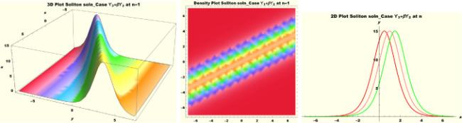
View original graphic|Download|PPT slide

Fig.1 Bright soliton wave profile of (3.21), $- 10 \leq x, y \leq 10$ at $t = 0$ for $n = 1$ .

View original graphic|Download|PPT slide

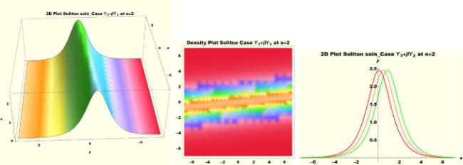
Fig.2 Bright soliton wave profile of (3.21), $- 10 \leq x, y \leq 10$ at $t = 0$ for $n = 2$ .

View original graphic|Download|PPT slide

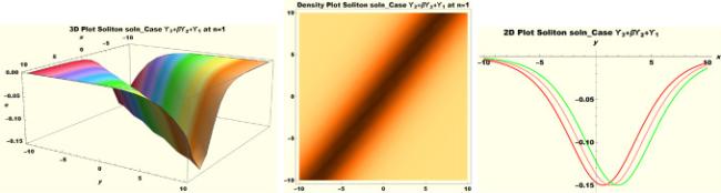
Fig.3 Dark soliton wave profile of (3.29), $- 10 \leq x, y \leq 10$ at $t = 1$ for $n = 1$ .

View original graphic|Download|PPT slide

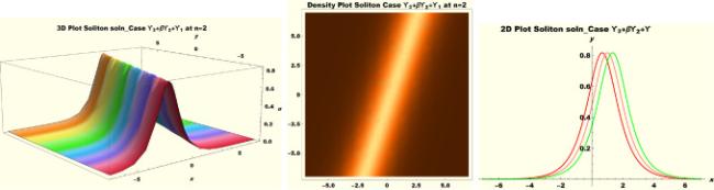
Fig.4 Bright soliton wave profile of (3.29), $- 7 \leq x, y \leq 7$ at $t = 1$ for $n = 2$ .

View original graphic|Download|PPT slide

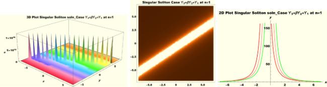
Fig.5 Multi-soliton wave structure of (3.30), $- 7 \leq x, y \leq 7$ at $t = - 2$ for $n = 1$ .

View original graphic|Download|PPT slide

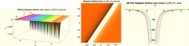
Fig.6 Multi-soliton wave structure of (3.30), $- 7 \leq x, y \leq 7$ at $t = - 2$ for $n = 2$ .

View original graphic|Download|PPT slide

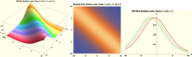
Fig.7 Bright soliton wave profile of (3.33), $- 10 \leq x, y \leq 10$ at $t = 0.3$ for $n = 1$ .

View original graphic|Download|PPT slide

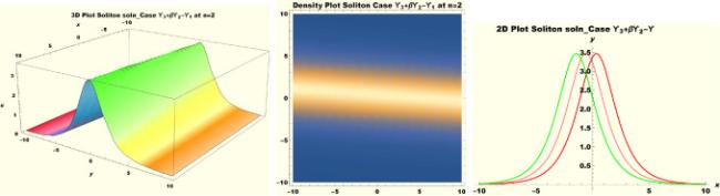
Fig.8 Bright soliton wave profile of (3.33), $- 10 \leq x, y \leq 10$ at $t = 0.3$ for $n = 2$ .

View original graphic|Download|PPT slide

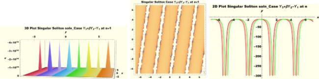
Fig.9 Multi-soliton wave profile of (3.34), $- 7 \leq x, y \leq 7$ at $t = - 0.8$ for $n = 1$ .

View original graphic|Download|PPT slide

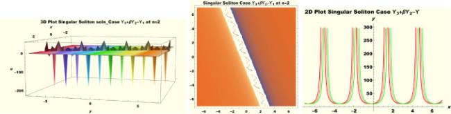
Fig.10 Multi-soliton wave profile of (3.34), $- 7 \leq x, y \leq 7$ at $t = - 0.8$ for $n = 2$ .

View original graphic|Download|PPT slide

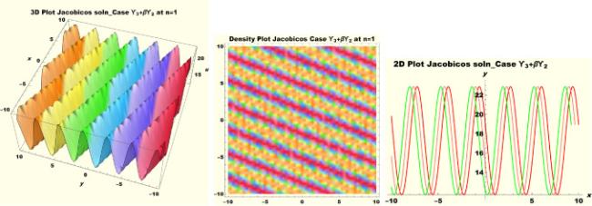
Fig.11 Smooth periodic wave profile of (4.43) with $- 10 \leq x, y \leq 10$ at $t = - 1$ .

View original graphic|Download|PPT slide

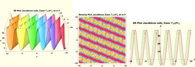
Fig.12 Smooth periodic wave profile of (4.44) with $- 10 \leq x, y \leq 10$ at $t = - 3$ .

View original graphic|Download|PPT slide

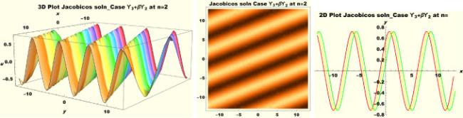
Fig.13 Smooth periodic wave profile of solution (4.48), $- 13 \leq x, y \leq 13$ at $t = 2$ .

View original graphic|Download|PPT slide

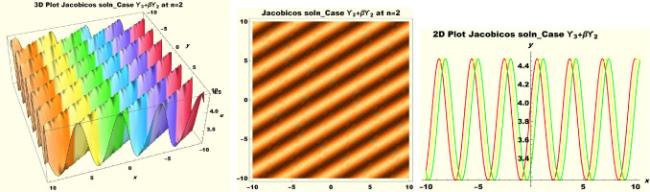
Fig.14 Smooth periodic wave profile of solution (4.49), $- 10 \leq x, y \leq 10$ at $t = 0$ .

View original graphic|Download|PPT slide

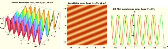
Fig.15 Smooth periodic wave profile of (4.53), $- 12 \leq x, y \leq 12$ at $t = - 5$ .

View original graphic|Download|PPT slide

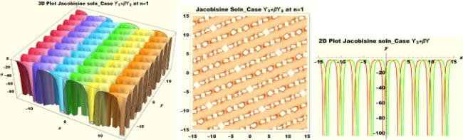
Fig.16 Singular periodic wave profile of (4.54), $- 15 \leq x, y \leq 15$ at $t = 10$ .

View original graphic|Download|PPT slide

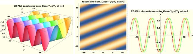
Fig.17 Smooth periodic wave profile of (4.58), $- 12 \leq x, y \leq 12$ at $t = 4$ .

View original graphic|Download|PPT slide

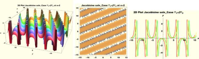
Fig.18 Singular periodic wave profile of (4.59), $- 15 \leq x, y \leq 15$ at $t = 2.3$ .

View original graphic|Download|PPT slide

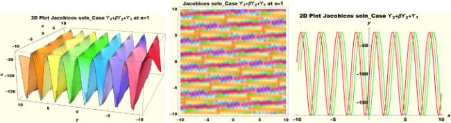
Fig.19 Smooth periodic wave profile of (4.64) with $- 10 \leq x, y \leq 10$ at $t = - 4.2$ .

View original graphic|Download|PPT slide

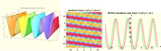
Fig.20 Smooth periodic wave profile of (4.65) with $- 13 \leq x, y \leq 13$ at $t = - 3.7$ .

via the selection of parametric values

β = 0.2

ω = 1.01

a = 1.03

b = 1

c = 1.00000000001

d = 2

e = 0

, with

t = - 3.7

as well as

- 13 \leq x, y \leq 13

. The numerical simulation of periodic soliton (4.66) occasions the diagrammatic representations in Fig. 21 with unalike constant values

β = 0.01

α = 0.2

a = 1.03

b = 1

c = 1.00000000001

d = 2

e = 0

, with

t = 6.2

View original graphic|Download|PPT slide

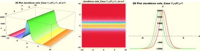
Fig.21 Bell shape wave profile of (4.66) with $- 10 \leq x, y \leq 10$ at $t = 6.2$ .

whereas on the

(x, y)

-plane,

(x, y) \in [- 10, 10]

. Moreover, the wave portrayal of cnoidal wave solution (4.70) is achieved in Fig. 22 through the use of variant parametric values designated as

β = 10

α = 13

ω = - 10

a = 10

c = 10.00000000001

d = 2

e = 1

, where variables

t = 20

and

- 10 \leq x, y \leq 10

. Fig. 23 reveals the wave motion of bright soliton solution (4.71) by invoking constant values

β = 0.1

α = 0.3

a = 1

c = 10

d = 2

e = 1.00000000001

, with variables

t = - 20

View original graphic|Download|PPT slide

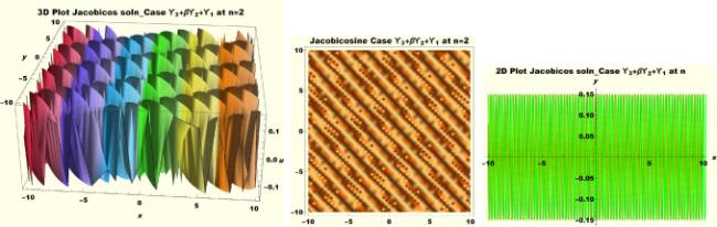
Fig.22 Periodic wave profile of (4.70) with $- 10 \leq x, y \leq 10$ at $t = 20$ .

View original graphic|Download|PPT slide

Fig.23 Bell shape wave profile of (4.71) with $- 10 \leq x, y \leq 10$ at $t = - 20$ .

whereas on the

(x, y)

-plane,

(x, y) \in [- 10, 10]

. Next, we examine the wave dynamics of snoidal wave solutions. Thus, solution (4.76) is represented via Fig. 24 with parametric values

α = 0.4

ω = 0.4

a = 5

b = 1

c = 0.1

d = 2

e = 1.00000000001

, with

t = 8.3

as well as

- 12 \leq x, y \leq 12

. Besides, we plot solution (4.77) in Fig. 25 by assigning

α = 1

ω = 0.6

a = 5

b = 1.00000000001

c = 0.1

d = 2

e = 1

, with

t = - 0.6

alongside

(x, y) \in [- 15, 15]

. Solution (4.78) is depicted in Fig. 26 through the dissimilar constant values

α = 0.3

β = - 0.9

ω = 0.3

a = 5

b = 1

c = - 0.1

d = 2

e = 1.00000000001

, whereas

t

assumes the same value and

(x, y)

, the same range. Periodic soliton (4.83) is plotted in Fig. 27 with

α = 0.4

ω = 0.4

a = 5

c = - 0.1

d = - 2

e = 1

, with

t = 0.2

View original graphic|Download|PPT slide

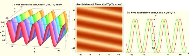
Fig.24 Smooth periodic wave profile of (4.76) with $- 12 \leq x, y \leq 12$ at $t = 8.3$ .

View original graphic|Download|PPT slide

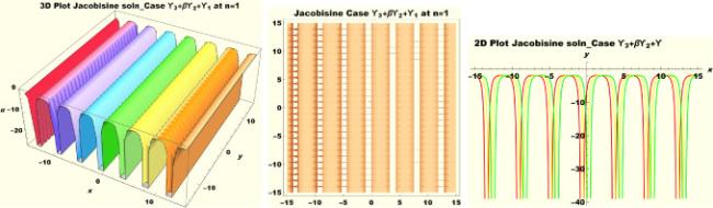
Fig.25 Singular periodic wave profile of (4.77) with $- 15 \leq x, y \leq 15$ at $t = - 0.6$ .

View original graphic|Download|PPT slide

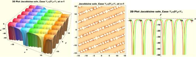
Fig.26 Singular periodic wave profile of (4.78) with $- 15 \leq x, y \leq 15$ at $t = - 0.6$ .

View original graphic|Download|PPT slide

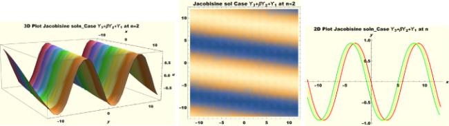
Fig.27 Smooth periodic wave profile of (4.83) with $- 12 \leq x, y \leq 12$ at $t = 0.2$ .

where

(x, y) \in [- 12, 12]

where solution (4.84) is portrayed in Fig. 28 using

β = 0.08

a = 5

c = 0.1

d = - 2

e = 1

, variable

t = 1.8

and

(x, y) \in [- 15, 15]

. We reveal the dynamics of snoidal wave solution (4.85) in Fig. 29 through

α = 0.7

β = 0.001

a = 0.1

c = 0

d = 0.02

e = 0.00000000001

, whereas

t = - 0.5

together with

(x, y) \in [- 10, 10]

. Furthermore, cnoidal wave solution (4.91) is depicted in Fig. 30 via constants

σ = 0.4

β = 0.2

ω = 0.7

a = 1

b = 1.00000000001

c = 1.000000001

d = 2

e = 0

, with

t = - 10

alongside

- 10 \leq x, y \leq 10

. In the same vein, periodic solution (4.91) is plotted in Fig. 31 through variant parametric values

σ = 0.5

β = 0.3

ω = 1.01

a = 1.03

b = 1.00000000001

c = 1

d = 2

e = 0

, where we have

t = 9

as well as

- 13 \leq x, y \leq 13

. In Fig. 32, we represent cnoidal wave (4.91) via constant values

σ = 0.6

β = 0.2

ω = 1.01

a = - 0.1

b = 10

c = 1

d = 2

e = 0

, where

t = - 6

and

- 10 \leq x, y \leq 10

. Besides, solitary wave solution (4.92) is furnished in Fig. 33 using

σ = 1

β = 0.6

ω = 1.05

a = 0.1

b = 1

c = 0

d = 2

e = 0.00000000001

, with

t = 0.7

alongside

- 10 \leq x, y \leq 10

. Solitary wave solution (4.99) is represented in Fig. 34 by utilizing parameters

σ = 0.3

β = 0.2

a = - 1

d = 2

e = 1

, whereas

t = 1

together with

(x, y) \in [- 10, 10]

. In addition to that cnoidal wave (4.100) is exhibited in Fig. 35 by invoking parametric values

σ = 0.3

β = 0.1

a = 1

b = 10

d = 2

e = 1.00000000001

, where

t = - 2

alongside

(x, y) \in [- 8, 8]

. We depict periodic soliton (4.101) in Fig. 36 via the use of

σ = 1

β = 0.1

a = 1

b = 100

d = 2

e = 1.00000000001

, whereas

t = 12

and

(x, y) \in [- 10, 10]

. Furthermore, solitary wave solution (4.107) is purveyed in Fig. 37 with dissimilar constants

σ = 0.4

β = 0.3

ω = 0.6

a = 5

b = 1

c = - 0.1

d = 2

e = 1.00000000001

, where we have

t = 0.3

along with

- 10 \leq x, y \leq 10

. Periodic solution (4.108) is exhibited in Fig. 38 with unalike constants

σ = 0.41

β = 0.3

ω = 0.8

a = 5

b = 1.00000000001

c = 0.1

d = 2

e = 1

, with variables

t = 0.22

together with

- 10 \leq x, y \leq 10

on the

(x, y)

-plane. The snoidal wave (4.109) plotted in Fig. 39 is achieved via choice of constants

σ = 0.41

β = 0.5

ω = 0.8

a = 5

b = 1

c = 0.1

d = 2

e = 1.00000000001

, whereas variable

t = 5.6

alongside

- 15 \leq x, y \leq 15

View original graphic|Download|PPT slide

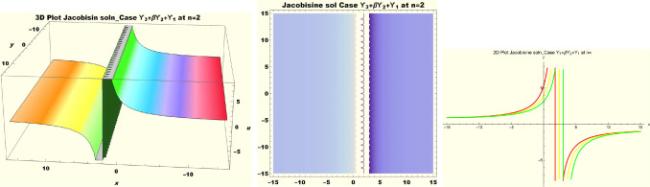
Fig.28 Singular periodic wave profile of (4.84) with $- 15 \leq x, y \leq 15$ at $t = 1.8$ .

View original graphic|Download|PPT slide

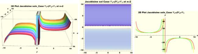
Fig.29 Singular periodic wave profile of (4.85) with $- 10 \leq x, y \leq 10$ at $t = - 0.5$ .

View original graphic|Download|PPT slide

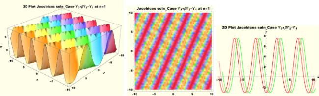
Fig.30 Periodic wave profile of (4.91) with $- 10 \leq x, y \leq 10$ at $t = - 10$ .

View original graphic|Download|PPT slide

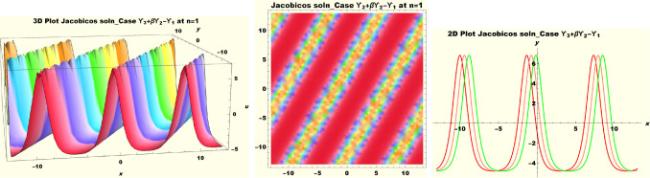
Fig.31 Periodic wave profile of (4.92) with $- 13 \leq x, y \leq 13$ at $t = 9$ .

View original graphic|Download|PPT slide

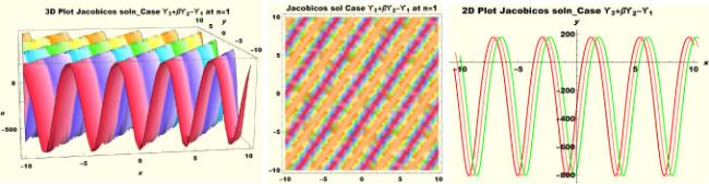
Fig.32 Periodic wave profile of (4.93) with $- 10 \leq x, y \leq 10$ at $t = - 6$ .

View original graphic|Download|PPT slide

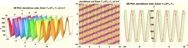
Fig.33 Periodic wave profile of (4.94) with $- 10 \leq x, y \leq 10$ at $t = 0.7$ .

View original graphic|Download|PPT slide

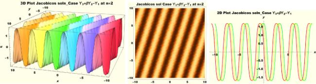
Fig.34 Periodic wave profile of (4.99) with $- 10 \leq x, y \leq 10$ at $t = 1$ .

View original graphic|Download|PPT slide

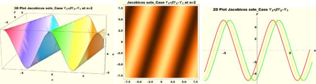
Fig.35 Periodic wave profile of (4.100) with $- 8 \leq x, y \leq 8$ at $t = - 2$ .

View original graphic|Download|PPT slide

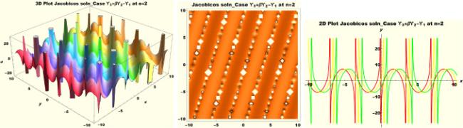
Fig.36 Singular periodic wave profile of (4.101) with $- 10 \leq x, y \leq 10$ at $t = 12$ .

View original graphic|Download|PPT slide

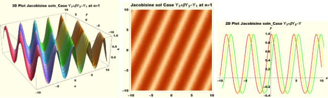
Fig.37 Smooth periodic wave profile of (4.107) with $- 10 \leq x, y \leq 10$ at $t = 0.3$ .

View original graphic|Download|PPT slide

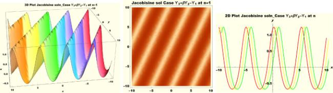
Fig.38 Smooth periodic wave profile of (4.108) with $- 10 \leq x, y \leq 10$ at $t = 0.22$ .

View original graphic|Download|PPT slide

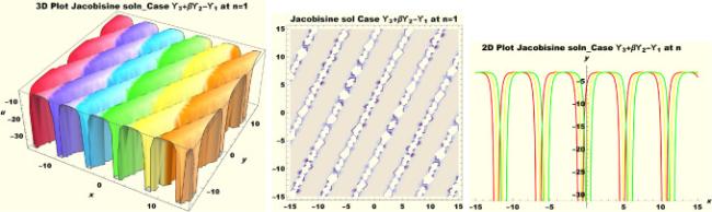
Fig.39 Singular periodic wave profile of (4.109) with $- 15 \leq x, y \leq 15$ at $t = 5.6$ .

Moreover, dynamics of snoidal wave (4.110) is numerically simulated thereby purveying Fig. 40 by engaging most beneficial parametric constant values

σ = 0.41

β = 0.5

ω = 0.1

a = 5

b = 1.00000000001

c = 0.1

d = 2

e = 1

, whereas we have variable

t = - 2.4

and also

(x, y) \in [- 15, 15]

. Fig. 41 depicts smooth periodic solution (4.115) using

σ = 0.4

β = 0.2

ω = 0.2

a = - 2

c = - 0.1

d = - 2

e = 1

, with variable

t = 20

and

(x, y) \in [- 12, 12]

on the

(x, y)

-plane. In the same vein, smooth snoidal wave (4.116) is portrayed in Fig. 42 with dissimilar constant values

β = 0.08

a = 5

b = 3.3

d = - 2

e = 1

, where

t = 30

and

- 15 \leq x, y \leq 15

. Finally, we simulate periodic soliton (4.117) numerically via

β = 1

a = 1

b = - 1

c = 0.2

d = 0.02

e = 0

, where we assign variable

t = 0

and

(x, y) \in [- 1, 1]

on the

(x, y)

-plane.

View original graphic|Download|PPT slide

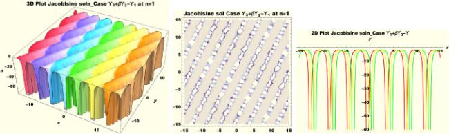
Fig.40 Singular periodic wave profile of (4.110) with $- 15 \leq x, y \leq 15$ at $t = - 2.4$ .

View original graphic|Download|PPT slide

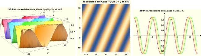
Fig.41 Smooth periodic wave profile of (4.115) with $- 12 \leq x, y \leq 12$ at $t = 20$ .

View original graphic|Download|PPT slide

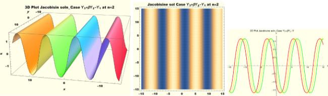
Fig.42 Smooth periodic wave profile of (4.116) with $- 15 \leq x, y \leq 15$ at $t = 30$ .

View original graphic|Download|PPT slide

Fig.43 Singular periodic wave profile of (4.117) with $- 1 \leq x, y \leq 1$ at $t = 0$ .

6. Applications of cnoidal and snoidal waves in ocean engineering and oceanography

In this study, we are aware that various solutions attained comprise copious cnoidal and snoidal waves which are solitary waves or periodic solitons. Cnoidal waves can be presented as an infinite sum of periodically repeated solitary waves. These waves have been comprehensively demonstrated through numerical simulations of the solutions using computer software by making adequate choices of parameters.

A solitary wave [7], [65], [66], [67] is the kind of wave propagating in the absence of any temporal evolution with regards to shape or size when it is viewed concerning the reference frame travelling with the group velocity existing in the wave. Furthermore, the envelope of the wave is possessive of one global peak whose decays occur far away from the peak. It is observed that solitary waves surface in various contexts that are inclusive of the elevation of the surface of the water as well as the intensity of light which is resident in optical fibres. In addition, a soliton is a nonlinear type of solitary wave which is possessive of an additional characteristic that the wave, after interacting with another soliton still conserves its permanent structure. For instance, in two solitons generating in the directions opposite to each other, successfully move through each other as it were without any breakage [68]. (See Figs. 44-45).

View original graphic|Download|PPT slide

Fig.44 Ocean's surface solitary wave triggered by atmosphere lower boundary's decreasing pressures [69].

View original graphic|Download|PPT slide

Fig.45 Schematic diagram of the life cycle of nonlinear internal waves in the region southeast of Hainan Island [70].

Solitons constitute a remarkable group of solutions related to some model equations. These equations comprise the Korteweg de-Vries as well as the Nonlinear Schrödinger equations. These equations are approximations, that are true under a confining set of criteria. The soliton results achieved from the model equation give us some understanding of the dynamical behaviour of solitary waves. Nevertheless, they are restrained by the criteria under which the model equations operate. A surrogate approach, relating directly to the precise equations where the model equations are constructed, gives an awareness of a larger class of solitary waves than those which are achieved via the model equations. Information with regards to the possible existence of a certain class of solitary waves can be achieved via a phase-plane formalism which is a common technique engaged in dynamical systems. Thus, a solitary wave, in this framework, corresponds to a homoclinic orbit that is existing in a spatial dynamical system. In addition, the occurrence of solitary waves is discovered in many diverse cases, which are determined, by their level of decay concerning the distance from their global peak. In consequence, a keen investigation of the tail regions, relative to their distance from the global peak, reveals that four possible cases of solitary waves can be achieved. Three of these cases include; the one secured via the steady-state solution of the Korteweg de-Vries equation. Secondly, a generalized solitary wave decays to non-zero oscillations with uniform amplitude as well as wave number. Thirdly, an envelope solitary wave, which fulfils the Nonlinear Schrödinger equation[68].

Moreover, solitary waves can be contemplated as a class of nonlinear, nonsinusoidal, more-or-less isolated waves which have complex shapes frequently occurring in nature. Internal waves are waves existing and also travelling within the interior of a given fluid. Such waves are very common as oscillations and they are visible in a two-layer fluid contained in a clear plastic box. The coherence of these waves is sustained. In the same vein, the visibility of the waves is conserved via nonlinear hydrodynamics that surface in imagery, as long quasilinear stripes. Besides, the signatures of internal waves are made conspicuous through current or wave interactions. In such a case, the related near-surface current to the internal wave modulates locally with regard to the height of the surface wave spectrum[71]. (See Fig. 45).

Ocean engineering is comprehensively defined as an area of technological investigation relating to the design alongside operations of man-made systems that is existing in the ocean as well as other marine bodies. In fact, it makes provision for essential interconnections that is existing among other disciplines of oceanography which consist of chemical together with physical oceanography, marine biology as well as marine geology and geophysics. The innovations in the instrumentation along with equipment design effectuated by ocean engineers have restructured the field of oceanography. In the same vein, the oceanographers' central point has been to drive the demand for design skills in conjunction with the technical expertise of ocean engineers. Moreover, unswervingly, ocean engineering incorporates diverse other areas of engineering which comprise a merge of mechanical, electrical, acoustical, chemical alongside civil engineering skills as well as techniques in consonance with a basic understanding of the way oceans operate (see the schematic diagram in Fig. 47). In addition to designing the building instruments that must outlive the wear and tear of persistent use, ocean engineers must also design instruments that can come through the harsh realities surrounding the ocean environment.

Hazardous events, which include rock falls or avalanches, rock slides, and landslides, frequently generate great, impulsive waves when they enter or are submerged in water bodies [73]. Therefore, these waves are then approximated through the use of solitary waves whose overwhelming potential damage with regard to the built environment has been investigated by researchers. In order to further deepen the understanding of solitary waves which run up a constant beach slope and also propagate over a subsequent horizontal plane can assist in minimizing as well as attenuating damage and the number of casualties that can be caused as a result of the damning effect of such a hazardous event [74]. The interaction exiting between structures alongside waves is a typical phenomenon in naval architecture as well as ocean engineering. Consequently, we present some relevance of solitary waves in oceanography and ocean engineering .

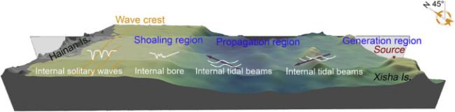
Oceanographers and acousticians have realized that shallow water internal solitary waves are a major topic of interest . The investigation into internal solitary waves found in ocean acoustic was motivated by the discovery of an anomalous frequency response of sound propagation measurements which was noticed in shallow water (see Fig. 46). The spatial, as well as temporal scales of internal bores and solitary waves that are induced by tides, are the type that can significantly affect the acoustic field via the structure of sound speed. The interaction between the acoustical field and the solitary wave train at certain frequencies can be quite significant. Various interactions that existed between the acoustical field, as well as the solitary wave train, can also emerge between the receiver and source. In [75], the scientist conducted theoretical research into the coupling of acoustical normal modes where the presence of solitary-wave-type disturbances was observed. They discovered that strong lateral gradients of sound speed in the waves occasioned the transfer of energy between various acoustical modes. The phase mode within the solitary wave packet differs with time scales of minutes. This eventually causes coupling and signal fluctuations at comparable time scales. Furthermore, right from the studies conducted by Zhou et al. [76], oceanographic alongside littoral acoustical experiments have been conducted on the synoptic as well as local scales, where the experiment fronts reveal that there was a prevalence of eddies, tidal effects, internal waves, mesoscale variability together with solitary waves. Surveys have also been conducted on the New England and New Jersey continental shelves[77].

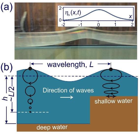
View original graphic|Download|PPT slide

Fig.46 Russell's solitary-wave solitons occur in shallow water channels, (a) as shown in a laboratory reconstruction of Russell's original observation. The inset is a typical localized solution of the Korteweg-de Vries equation for extremely shallow water. (b) In deep water, waves propagate (from left to right), whereas water particles orbit in circles around their average position. The diameter of the circular orbits shrinks gradually with increasing distance from the surface down to half the wavelength $L$ . In shallow waters with depth $h < L / 2$ , the orbits become elliptical and essentially flat at the bottom of the tank or seabed [72].

View original graphic|Download|PPT slide

Fig.47 A simplified concept of the main wave transformation and attenuation processes which must be considered by coastal engineers in designing coastal defence schemes [78].

7. Conservation laws of 3D-gextQZKe (1.4)

In this section we construct the conservation laws for the 3D-gextQZKe (1.4). We achieve that by using Noether's theorem.

7.1. Construction of conservation laws using the Noether theorem

This subsection begins with the employment of the well-celebrated Noether theorem [79] to derive the conservation laws of the 3D-gextQZKe (1.4). Here we discovered that (1.4) does not admit any Lagrangian in its current state and as such possesses no variational principle. Notwithstanding, to circumvent that we engage the transformation

u = U_{x}

and interestingly, we secure a fourth-order form of Eq. (1.4) structured as

(7.118)

E^{*} = U_{t x} + a U_{x}^{n} U_{x x} + b U_{x x x x} + c U_{x y y y} + d U_{x x y y} + e U_{x x x y} = 0,

which readily has a Lagrangian. Hence, we present a Lemma to that effect.

Lemma 7.1. The 3D-gextQZKe (1.4) manifests the Euler-Lagrange equation having the functional

(7.119)

J (U) = \int_{0}^{\infty} \int_{0}^{\infty} \int_{0}^{\infty} L (x, y, t, U_{x}, U_{t}, U_{x x}, U_{x y}, U_{y y}) d x d y d t,

where the conforming function of Lagrange

L

is expressed as

(7.120)

\begin{matrix} L & = & - \frac{1}{2} U_{t} U_{x} - \frac{a}{(n + 1) (n + 2)} U_{x}^{n + 2} + \frac{b}{2} U_{x x}^{2} + \frac{c}{2} U_{x y} U_{y y} \\ + \frac{d}{2} U_{x x} U_{y y} + \frac{e}{2} U_{x x} U_{x y} . \end{matrix}

One can readily proof that the second-order Lagrangian for the fourth-order PDE (7.118) which is given in (7.120) satisfies the Euler-Lagrangian equation

δ L / δ U = 0 = E^{*}

as envisaged, by utilizing the standard Euler operator

δ / δ U

expressed as

\frac{δ}{δ U} = \frac{\partial}{\partial U} - D_{t} \frac{\partial}{\partial U_{t}} - D_{x} \frac{\partial}{\partial U_{x}} + D_{t}^{2} \frac{\partial}{\partial U_{t t}} + D_{x}^{2} \frac{\partial}{\partial U_{x x}} + D_{t} D_{x} \frac{\partial}{\partial U_{t x}} - \dots,

where total derivatives

D_{t}

D_{x}

and

D_{y}

can be calculated from (2.10). In a bid to secure the variational symmetries

Σ = ξ^{1} \partial / \partial x + ξ^{2} \partial / \partial y + ξ^{3} \partial / \partial t + η \partial / \partial U

which is correspondent to the stated Lagrangian (7.120), we shall utilize the invariance condition

(7.121)

{Pr}^{(2)} Σ L + L [D_{x} (ξ^{1}) + D_{y} (ξ^{2}) + D_{t} (ξ^{3})] = D_{x} (B^{x}) + D_{y} (B^{y}) + D_{t} (B^{t}),

where second prolongation

{Pr}^{(2)} Σ

is defined as

{Pr}^{(2)} Σ = ζ_{t} \frac{\partial}{\partial U_{t}} + ζ_{x} \frac{\partial}{\partial U_{x}} + ζ_{y} \frac{\partial}{\partial U_{y}} + ζ_{x x} \frac{\partial}{\partial U_{x x}} + ζ_{x y} \frac{\partial}{\partial U_{x y}} + ζ_{y y} \frac{\partial}{\partial U_{y y}},

We notice that coefficient functions

ξ^{1}

ξ^{2}

ξ^{3}

η

as well as gauge functions

B^{x}

B^{y}

and

B^{t}

are depending on

(x, y, t, U)

. To determine the Noether symmetry generators

Σ

, we expand invariance condition (7.121) and separate the monomials and that furnishes the sixty-four system of linear PDEs, which are

\begin{matrix} ξ_{U}^{1} = 0, ξ_{x}^{3} = 0, ξ_{U U}^{3} = 0, η_{x} = 0, ξ_{U x}^{3} = 0, ξ_{t}^{3} = 0, ξ_{U}^{3} = 0, \\ ξ_{U U}^{1} = 0, ξ_{U}^{2} = 0, ξ_{y}^{1} = 0, ξ_{U U}^{2} = 0, ξ_{U x}^{3} = 0, ξ_{U x}^{1} = 0, \\ ξ_{U y}^{1} = 0, ξ_{x}^{1} = 0, ξ_{t}^{2} = 0, ξ_{U}^{3} = 0, B_{U}^{y} = 0 4 b ξ_{U x}^{1} + e ξ_{U y}^{1} = 0, \\ ξ_{U}^{1} + B_{U}^{t} = 0, e η_{x x} + c η_{y y} = 0, ξ_{U}^{3} + B_{U}^{t} = 0, c η_{x y} + d η_{x x} = 0, \\ η_{U U} - 2 ξ_{U y}^{3} = 0, c ξ_{U y}^{1} + 2 d ξ_{U x}^{1} = 0, c ξ_{x y}^{1} + d ξ_{x x}^{1} = 0, c ξ_{U}^{2} + d ξ_{U}^{3} = 0, \\ c ξ_{U}^{2} + 3 d ξ_{U}^{3} = 0, c ξ_{U U}^{2} + d ξ_{U U}^{3} = 0, \\ 2 d ξ_{x}^{1} + c ξ_{y}^{1} = 0, η_{U U} - 2 ξ_{U x}^{2} = 0, \\ e ξ_{x}^{1} + 2 d ξ_{y}^{1} = 0, e ξ_{y}^{1} + 4 b ξ_{x}^{1} = 0, \\ e ξ_{U x}^{1} + 2 d ξ_{U y}^{1} = 0, e ξ_{x x}^{1} + c ξ_{y y}^{1} = 0, \\ e ξ_{U}^{2} + b ξ_{U}^{3} = 0, e ξ_{U U}^{2} + 2 b ξ_{U U}^{3} = 0, \\ e ξ_{U}^{3} + d ξ_{U}^{2} = 0, e ξ_{U}^{3} + 3 d ξ_{U}^{2} = 0, \\ e ξ_{x}^{3} + c ξ_{y}^{2} = 0, e ξ_{U U}^{3} + d ξ_{U U}^{2} = 0, e ξ_{U x}^{3} + c ξ_{U y}^{2} = 0, η_{t} + 2 B_{U}^{x} = 0, \\ B_{y}^{y} + B_{x}^{x} = 0, d η_{U U} - c ξ_{U y}^{2} - 2 d ξ_{U x}^{2} = 0, c η_{U x} - c ξ_{x y}^{3} - d ξ_{x x}^{3} = 0, \\ 2 e η_{U x} - e ξ_{x x}^{2} - c ξ_{y y}^{2} = 0, 2 b η_{x x} + e η_{x y} + d η_{y y} = 0, \\ e ξ_{x y}^{1} + d ξ_{y y}^{1} + 2 b ξ_{x x}^{1} = 0, \\ 2 b η_{U U} - e ξ_{U y}^{2} - 4 b ξ_{U x}^{2} = 0, d η_{U U} - e ξ_{U x}^{3} - 2 d ξ_{U y}^{3} = 0, \\ 2 c η_{U y} - e ξ_{x x}^{3} - c ξ_{y y}^{3} = 0, \\ (n + 1) ξ_{U}^{1} + B_{U}^{t} = 0, B_{t}^{t} - ξ_{y}^{3} - 2 η_{U} = 0, \\ c η_{U U} - c ξ_{U x}^{2} - c ξ_{U y}^{3} - 2 d ξ_{U x}^{3} = 0, \\ c η_{U y} - c ξ_{x y}^{2} + 2 d η_{U x} - d ξ_{x x}^{2} = 0, \\ c ξ_{t}^{1} - c B_{t}^{t} - 2 d ξ_{x}^{3} + 2 c η_{U} - 2 c ξ_{y}^{3} = 0, \\ e η_{U U} - e ξ_{U x}^{2} - e ξ_{U y}^{3} - 2 d ξ_{U y}^{2} - 4 b ξ_{U x}^{3} = 0, \\ e η_{U x} - e ξ_{x y}^{3} + 2 d η_{U y} - d ξ_{y y}^{3} - 2 b ξ_{x x}^{3} = 0, \\ e η_{U y} - e ξ_{x y}^{2} - d ξ_{y y}^{2} + 4 b η_{U x} - 2 b ξ_{x x}^{2} = 0, \\ b ξ_{t}^{1} + b ξ_{y}^{3} - b B_{t}^{t} - e ξ_{y}^{2} + 2 b η_{U} - 3 b ξ_{x}^{2} = 0, \\ e ξ_{t}^{1} - e B_{t}^{t} - 2 d ξ_{y}^{2} + 2 e η_{U} - 2 e ξ_{x}^{2} - 4 b ξ_{x}^{3} = 0, \\ (n + 2) (ξ_{x}^{2} - η_{U}) - ξ_{t}^{1} - ξ_{x}^{2} - ξ_{y}^{3} + B_{t}^{t} = 0, \\ d ξ_{t}^{1} - d B_{t}^{t} - e ξ_{x}^{3} + 2 d η_{U} - d ξ_{x}^{2} - d ξ_{y}^{3} - c ξ_{y}^{2} = 0 . \end{matrix}

From the system of PDEs, we secure the values of the coefficient functions as

\begin{matrix} ξ^{1} = \frac{1}{3} C_{1} x + C_{2}, ξ^{2} = \frac{1}{3} C_{1} y + C_{3}, \\ ξ^{3} = C_{1} t + C_{4}, η = \frac{n - 2}{3 n} C_{1} U + G (t) y + E (t), \\ B^{x} = - \frac{1}{2} G^{'} (t) y U - \frac{1}{2} E^{'} (t) U + F^{1} (y, t) - \int F_{y}^{2} d x, \\ B^{y} = F^{3} (x, y, t), B^{t} = (\frac{3 n - 4}{3 n}) C_{1} t + F^{4} (x, y) . \end{matrix}

Functions

F^{1}, F^{2}

and

F^{3}

are set to zero due to the reason that they contribute to the trivial part of the conserved vectors. Thus, the coefficient functions yields the six Noether symmetries alongside their respective gauge functions, viz.,

(7.122)

\begin{matrix} Σ_{1} = \frac{\partial}{\partial x}, B^{t} = 0, B^{x} = 0, B^{y} = 0, \\ Σ_{2} = \frac{\partial}{\partial y}, B^{t} = 0, B^{x} = 0, B^{y} = 0, \\ Σ_{3} = \frac{\partial}{\partial t}, B^{t} = 0, B^{x} = 0, B^{y} = 0, \\ Σ_{4} = t \frac{\partial}{\partial t} + \frac{1}{3} x \frac{\partial}{\partial x} + \frac{1}{3} y \frac{\partial}{\partial y} + (\frac{n - 2}{3 n}) U \frac{\partial}{\partial U}, \\ B^{t} = (\frac{3 n - 4}{3 n}) t, B^{Σ} = 0, B^{y} = 0 . \\ Σ_{E} = E (t) \frac{\partial}{\partial U}, B^{t} = 0, B^{x} = - \frac{1}{2} E^{'} (t) U, B^{y} = 0, \\ Σ_{G} = G (t) y \frac{\partial}{\partial U}, B^{t} = 0, B^{x} = - \frac{1}{2} G^{'} (t) y U, B^{y} = 0 . \end{matrix}

The respective conserved vectors [26], [80] for the Noether symmetry operators

Σ_{1}, \dots, Σ_{G}

associated with Lagrangian (7.120) can be secured from [80]

(7.123)

C^{i} = N^{i} (L) - B^{i}, i = 1, \dots, q,

in such a way that condition

D_{t} C^{t} + D_{x} C^{x} + D_{y} C^{y} = 0

, holds. The Noether operator

N^{i}

given in (7.123) is expressed as

(7.124)

N^{i} = ξ^{i} + W^{α} \frac{δ}{δ U_{i}^{α}} + \sum_{s \geq 1} D_{i_{1}} \dots D_{i_{1}} (W^{α}) \frac{δ}{δ U_{i_{1} i_{2} \dots i_{s}}^{α}}, α = 1, \dots, m,

with

q

and

m

representing the total number of independent and dependent variables respectively. The Euler-Lagrange operators with respect to derivatives of

U^{α}

is achieved from

(7.125)

\begin{matrix} \frac{δ}{δ U^{α}} & = & \frac{\partial}{\partial U^{α}} + \sum_{s \geq 1} (- 1)^{s} D_{i_{1}} \dots D_{i_{s}} \frac{δ}{δ U_{i_{1} i_{2} \dots i_{s}}^{α}}, \\ i & = & 1, \dots, q, α = 1, \dots, m, \end{matrix}

by substituting

U^{α}

with the corresponding derivatives. For instance,

(7.126)

\begin{matrix} \frac{δ}{δ U_{i}^{α}} & = & \frac{\partial}{\partial U_{i}^{α}} + \sum_{s \geq 1} (- 1)^{s} D_{j_{1}} \dots D_{j_{s}} \frac{δ}{δ U_{i j_{1} j_{2} \dots j_{s}}^{α}}, \\ j & = & 1, \dots, q, α = 1, \dots, m . \end{matrix}

Utilizing (7.120), (7.122) and (7.123), we generate local and nonlocal conserved vectors for respective generators

Σ_{1}

Σ_{2}

Σ_{3}

Σ_{4}

Σ_{E}

and

Σ_{G}

\begin{matrix} C_{1}^{t} = & \frac{1}{2} u^{2}, \\ C_{1}^{x} = & \frac{a}{n + 2} u^{n + 2} + \frac{1}{2} (- b u_{x}^{2} + d u u_{y y} + e (u u_{x y} - u_{x} u_{y})) + b u u_{x x}, \\ C_{1}^{y} = & c u u_{y y} + \frac{1}{2} (e u u_{x x} - c u_{y}^{2} + d (u u_{x y} - u_{x} u_{y})); \\ C_{2}^{t} = & \frac{1}{2} u \int u_{y} d x \\ C_{2}^{x} = & (\frac{1}{2} \int u_{t} d x + \frac{a}{n + 1} u^{n + 1} + b u_{x x} + \frac{1}{2} e u_{x y} + \frac{1}{2} d u_{y y}) \int u_{y} d x \\ - \frac{1}{2} (e u_{y}^{2} + [e u_{x} + d u_{y} + c \int u_{y y} d x] \int u_{y y} d x) - b u_{x} u_{y}, \\ C_{2}^{y} = & - \frac{a}{(n + 1) (n + 2)} u^{n + 2} + \frac{1}{2} (- u \int u_{t} d x + b u_{x}^{2} + e u_{x} u_{y}) \\ + (c u_{y y} + \frac{1}{2} e u_{x x} + \frac{1}{2} d u_{x y}) \int u_{y} d x; \\ C_{3}^{t} = & - \frac{a}{(n + 1) (n + 2)} u^{n + 2} + \frac{1}{2} (b u_{x}^{2} + e u_{x} u_{y} + c u_{y} \int u_{y y} d x), \\ + \frac{1}{2} d u_{x} \int u_{y y} d x, \\ C_{3}^{x} = & (\frac{1}{2} \int u_{t} d x + \frac{a}{n + 1} u^{n + 1} + b u_{x x} + \frac{1}{2} e u_{x y} + \frac{1}{2} d u_{y y}) \int u_{t} d x \\ - \frac{1}{2} [e u_{y} u_{t} + (e u_{x} + c \int u_{y y} d x) \int u_{y t} d x] - b u_{t} u_{x} \\ - \frac{1}{2} d u_{t} \int u_{y y} d x, \\ C_{3}^{y} = & (\frac{1}{2} e u_{x x} + c u_{y y} + \frac{1}{2} d u_{x y}) \int u_{t} d x - \frac{1}{2} (c u_{y} + d u_{x}) \int u_{y t} d x; \\ C_{4}^{t} = & \frac{1}{2} ((c t u_{y} + d t u_{x}) \int u_{y y} d x + b t u_{x}^{2} + e t u_{x} u_{y} - \frac{n - 2}{3 n} \int u d x) \\ - \frac{a}{(n + 1) (n + 2)} u^{n + 2} t + \frac{1}{3} (\frac{1}{2} y u \int u_{y} d x + \frac{1}{2} x u^{2} - \frac{3 n - 4}{n} t), \\ C_{4}^{x} = & \frac{1}{3} (\frac{a}{n + 2} x u^{n + 2} - \frac{1}{2} b x u_{x}^{2} + b x u u_{x x} + \frac{1}{2} d x u u_{y y} + \frac{1}{2} e x u u_{x y}) \\ + \frac{1}{2} (- \frac{n - 2}{3 n} \int u d x + t \int u_{t} d x + \frac{1}{3} y \int u_{y} d x + \frac{a}{n + 1} u^{n + 1} t) \int u_{t} d x \\ - \frac{1}{3} (\frac{a (n - 2)}{n (n + 1)} u^{n + 1} + \frac{(n - 2)}{n} b u_{x x} + \frac{(n - 2)}{2 n} d u_{y y} + \frac{(n - 2)}{2 n} e u_{x y}) \int u d x \\ + \frac{1}{3} (\frac{a}{n + 1} y u^{n + 1} + b y u_{x x} + \frac{1}{2} d y u_{y y} + \frac{1}{2} e y u_{x y} + \frac{c}{n} \int u_{y y}) \int u_{y} d x \\ + \frac{1}{2} t (2 b u_{x x} + d u_{y y} + e u_{x y}) \int u_{t} d x - \frac{2}{3 n} b u u_{x} - b t u_{t} u_{x} - \frac{1}{3} b y u_{x} u_{y} \\ - \frac{1}{2} (\frac{2}{3 n} d u + d t u_{t} + \frac{1}{3} d y u_{y} + c t \int u_{y t} d x + \frac{1}{3} c y \int u_{y y} d x) \int u_{y y} d x \\ - \frac{1}{3} (\frac{e}{n} u u_{y} + \frac{3}{2} e t u_{t} u_{y} + \frac{1}{2} e y u_{y}^{2} + \frac{e}{n} u_{x} \int u_{y} d x + \frac{3}{2} e t u_{x} \int u_{y t} d x) \\ - \frac{1}{6} e (x u_{x} u_{y} + y u_{x} \int u_{y y} d x), \\ C_{4}^{y} = & \frac{1}{3} (3 c t u_{y y} - \frac{1}{2} y u + \frac{3}{2} e t u_{x x} + \frac{3}{2} d t u_{x y}) \int u_{t} d x + \frac{1}{6} (b y u_{x}^{2} + e y u_{x} u_{y}) \\ - \frac{1}{3} (\frac{a}{(n + 1) (n + 2)} y u^{n + 2} + \frac{n - 2}{n} c u_{y y} \int u d x - c x u u_{y y} - \frac{1}{2} e x u u_{x x}) \\ + \frac{1}{3} (c y u_{y y} + \frac{1}{2} e y u_{x x} + \frac{1}{2} d y u_{x y} - \frac{c}{n} u_{y} - \frac{d}{n} u_{x}) \int u_{y} d x + \frac{1}{6} d x u u_{x y} \\ - \frac{(n - 2)}{6 n} (e u_{x x} + d u_{x y}) \int u d x - \frac{1}{2} t (c u_{y} + d u_{x}) \int u_{y t} d x - \frac{1}{6} c x u_{y}^{2} \\ - \frac{1}{6} d x u_{x} u_{y}; \\ C_{E}^{t} = & - \frac{1}{2} E (t) u, \\ C_{E}^{x} = & - (\frac{1}{2} \int u_{t} d x + \frac{a}{n + 1} u^{n + 1} + b u_{x x} + \frac{1}{2} (d u_{y y} + e u_{x y})) E (t) \\ + \frac{1}{2} E^{'} (t) \int u d x, \\ C_{E}^{y} = & - \frac{1}{2} (e u_{x x} + 2 c u_{y y} + d u_{x y}) E (t); \\ C_{G}^{t} = & - \frac{1}{2} G (t) y u, \\ C_{G}^{x} = & - (\frac{1}{2} \int u_{t} d x + \frac{a}{n + 1} u^{n + 1} + b u_{x x} + \frac{1}{2} (d u_{y y} + e u_{x y})) G (t) y \\ + \frac{1}{2} (e G (t) u_{x} + c G (t) \int u_{y y} d x + G^{'} (t) y \int u d x), \\ C_{G}^{y} = & - \frac{1}{2} (e u_{x x} + 2 c u_{y y} + d u_{x y}) G (t) y + \frac{1}{2} (c u_{y} + d u_{x}) G (t) . \end{matrix}

8. Conclusions

In this paper, we carried out a comprehensive investigation on a generalized extended (2+1)-dimensional quantum Zakharov-Kuznetsov equation with power-law nonlinearity (1.4) in oceanography and ocean engineering. The concept of the Lie group theory was engaged in achieving the task. In consequence, four-dimensional Lie algebra associated with (1.4) was gained. Besides, we constructed a 1-D optimal system of Lie subalgebras corresponding to the secured symmetries which were invoked to achieve various classical solutions for Eq. (1.4) through symmetry reductions as well as direct integration approach. Besides, the Jacobi functions expansion approach was engaged in securing general solutions to the underlying equation for some particular cases of

n

. The solutions contain bright, compact-type, dark, singular, non-topological and periodic solitons which represent both the bounded and unbounded solution-type related to the underlying equation. Moreover, to complete the solutions, we depicted the dynamics of the results with suitable graphical representations through numerical simulation using a computer software package. Sequel to that, applications of cnoidal and snoidal waves which were abundantly obtained in the course of the study were outlined in oceanography and ocean engineering fields. Furthermore, we constructed the conservation laws of (1.4) by imploring Noether's theorem of conserved quantities. These conservation laws are expressed in terms of both local and nonlocal conserved vectors. The nonlocal conserved vectors are the first integrals associated with the variational principle secured. In addition, conservations of energy and momentum which are highly applicable in theoretical physics are obtained in the study. In consequence of the aforementioned, the various results gained in this research work could be of interest to scientists in oceanography and theoretical physics as well as ocean and coastal engineers.

8.1. Future scope

Some of the achieved soliton solutions and various other results which include the conserved currents have diverse applications in physical sciences and some other engineering fields including plasma physics, mathematical physics, coastal science and engineering, solitons dynamics, and a wide range of other nonlinear sciences as well as engineering physics. In consequence, in the future, the dynamics of various soliton solutions could contribute to a broad-gauge theory to delineate the experience of the intricated diversity in diverse nonlinear physical systems. In the same vein, due to the fact that the evolutionary character of soliton solutions has invigorated outstanding research alongside development in a vast range of fields, it will be of great interest to examine the potential advantages of interactions that could exist between cnoidal-snoidal waves and that of the dynamical behaviour of mixed solitons (singular and non-singular).

Declaration of Competing Interest

The authors declare that they have no known competing financial interests or personal relationships that could have appeared to influence the work reported in this paper.

The authors declare the following financial interests/personal relationships which may be considered as potential competing interests:

No financial interests/personal relationships which may be considered as potential competing interests.

Acknowledgements

The author would like to thank the editor of the journal as well as the anonymous reviewers for their generous time in providing detailed comments along with suggestions that assisted in improving the paper.

References

Publishing order | Descend order by publishing year | Descend order by cited within

[1]	O.D. Adeyemo, C.M. Khalique. Symmetry (Basel), 14 (2022), p. 83 DOI: 10.3390/sym14010083

[2]	X.Y. Gao. Appl. Math. Lett., 91 (2019), pp. 165-172

[3]	O.D. Adeyemo, T. Motsepa, C.M. Khalique. Alex. Eng. J., 61 (2022), pp. 185-194

[4]	C.M. Khalique, O.D. Adeyemo. Results Phys., 18 (2020), p. 103197

[5]	X.X. Du, B. Tian, Q.X. Qu, Y.Q. Yuan, X.H. Zhao. solitons, self-adjointness and conservation laws of the modified Zakharov-Kuznetsov equation in an electron-positron-ion magnetoplasma, Chaos Solitons Fract., 134 (2020), p. 109709

[6]	C.R. Zhang, B. Tian, Q.X. Qu, L. Liu, H.Y. Tian. Z. Angew. Math. Phys., 71 (2020), pp. 1-19

[7]	C.M. Khalique, O.D. Adeyemo. J. Ocean Eng. Sci.(2021), p. 106393.

[8]	A.H. Salas, C.A. Gomez. Math. Probl. Eng. (2010), p. 2010

[9]	M.S. Osman, A.M. Wazwaz. Math. Method. Appl. Sci., 42 (2019), pp. 6277-6283 DOI: 10.1002/mma.5721

[10]	M.S. Osman. Nonlinear Dynam., 96 (2019), pp. 1491-1496 DOI: 10.1007/s11071-019-04866-1

[11]	M.G. Hafez, M. Kauser, M.T. Akter. J. Math. Comput. Sci., 4 (2014), pp. 2582-2593

[12]	M.A. Akbar, N.H.M. Ali. Springerplus, 3 (2014), p. 344

[13]	N.A. Kudryashov. Optik (Stuttg), 183 (2019), pp. 642-649

[14]	C.L. Zheng, J.P. Fang. Chaos Soliton Fract., 27 (2006), pp. 1321-1327

[15]	X.Y. Wen. Appl. Math. Comput., 217 (2010), pp. 1367-1375

[16]	A.M. Wazwaz. Partial Differential Equations. CRC Press, Boca Raton, Florida, USA (2002)

[17]	C. Chun, R. Sakthivel. Comput. Phys. Commun., 181 (2010), pp. 1021-1024

[18]	C.H. Gu. Soliton Theory and Its Application. Zhejiang Science and Technology Press, Zhejiang (1990)

[19]	X. Zeng, D.S. Wang. Appl. Math. Comput., 212 (2009), pp. 296-304

[20]	A.J.M. Jawad, M. Mirzazadeh, A. Biswas. Pramana, 83 (2014), pp. 457-471

[21]	N.A. Kudryashov, N.B. Loguinova. Appl. Math. Comput., 205 (2008), pp. 396-402

[22]	R. Hirota. The Direct Method in Soliton Theory. Cambridge University Press, Cambridge (2004)

[23]	L.V. Ovsiannikov. Group Analysis of Differential Equations. Academic Press, New York (1982)

[24]	G.W. Bluman, S. Kumei. Symmetries and Differential Equations. Springer-Verlag, New York (1989)

[25]	P.J. Olver. Applications of Lie Groups to Differential Equations, second ed. Springer-Verlag, Berlin (1993)

[26]	N.H. Ibragimov, CRC Handbook of Lie Group Analysis of Differential Equations, Vols 1-3, CRC Press, Boca Raton, Florida, 1994-1996.

[27]	N.H. Ibragimov. Elementary Lie Group Analysis and Ordinary Differential Equations. John Wiley & Sons, Chichester, NY (1999)

[28]	L. Zhang, C.M. Khalique. Discrete and Continuous dynamical systems Series S, 11 (4) (2018), pp. 777-790

[29]	M. Wang, X. Li, J. Zhang. Phys. Lett. A, 24 (2005), pp. 1257-1268

[30]	V.B. Matveev, M.A. Salle. Darboux Transformations and Solitons. Springer, New York (1991)

[31]	Y. Chen, Z. Yan. Chaos Solitons Fract., 26 (2005), pp. 399-406

[32]	N.A. Kudryashov. Chaos Solitons Fract., 24 (2005), pp. 1217-1231

[33]	J.H. He, X.H. Wu. Chaos Solitons Fract., 30 (2006), pp. 700-708

[34]	R. Sakthivel, C. Chun, J. Lee. Z. Naturforsch. A, 65 (2010), pp. 633-640 DOI: 10.1515/zna-2010-8-903

[35]	A.M. Wazwaz. Appl. Math. Comput., 169 (2005), pp. 321-338

[36]	J. Hu. Phys. Lett. A, 287 (2001), pp. 81-89

[37]	A. Biswas, A.J.M. Jawad, W.N. Manrakhan. Opt. Laser Technol., 44 (2012), pp. 2265-2269

[38]	A.M. Wazwaz. J. Nat. Sci. Math., 1 (2007), pp. 1-13

[39]	V.E. Zakharov, E.A. Kuznetsov. Zhurnal Eksp. Teoret.Fiz, 66 (1974), pp. 594-597

[40]	S.A. Khan, W. Masood. Phys.Plasmas, 15 (2008), p. 062301

[41]	B.S. Ahmed, E. Zerrad, A Math. Proc. Rom. Acad. Ser. A Math. Phys. Tech. Sci. Inf. Sci., 14 (2013), pp. 281-286

[42]	E.V. Krishnan, A. Biswas. Phys. wave phenom., 18 (2010), pp. 256-261

[43]	M.A. Abdou. Nonlinear Sci. Lett. B, 1 (2011), pp. 99-110

[44]	A.M. Wazwaz. Commun. Nonlinear Sci. Numer. Simul., 10 (2005), pp. 597-606

[45]	A.M. Wazwaz. the modified ZK equation, and its generalized forms, Commun. Nonlinear Sci. Numer. Simul., 13 (2008), pp. 1039-1047

[46]	A. Biswas. Phys. Lett. A, 373 (2009), pp. 2931-2934

[47]	D.M. Mothibi, C.M. Khalique. Symmetry (Basel), 7 (2015), pp. 949-961 DOI: 10.3390/sym7020949

[48]	G.W. Wang, T.Z. Xu, S. Johnson. Astrophys. Space Sci., 349 (2014), pp. 317-327 DOI: 10.1007/s10509-013-1659-z

[49]	A. Wazwaz. Phys. Scr., 85 (2012), p. 025006 DOI: 10.1088/0031-8949/85/02/025006

[50]	Y.L. Jiang, Y. Lu, C. Chen. J. Nonlinear Math. Phys., 23 (2016), pp. 157-166

[51]	G.W. Bluman, S. Kumei. Symmetries and Differential Equations, Applied Mathematical Science. Springer, Berlin (1989)

[52]	J.G. O'Hara, C. Sophocleous, P.G.L. Leach. J. Eng. Math., 82 (2013), pp. 67-75 DOI: 10.1007/s10665-012-9595-4

[53]	T. Chaolu, G. Bluman. J. Math. Anal. Appl., 411 (2014), pp. 281-296

[54]	R.K. Gupta, K. Singh. Commun. Nonlinear. Sci. Numer. Simul., 16 (2011), pp. 4189-4196

[55]	R. Jiwari, V. Kumar, K. Ram, S.A. Ali. Int. J. Numer. Method. H., 27 (2017), pp. 1332-1350 DOI: 10.1108/hff-04-2016-0145

[56]	R.K. Gupta, V. Kumar, R. Jiwari. Nonlinear Dyn., 79 (2014), pp. 455-464 DOI: 10.1007/978-3-662-45937-9_45

[57]	L. Kaur, R.K. Gupta. Math. Method. Appl. Sci., 36 (2013), pp. 584-600 DOI: 10.1002/mma.2617

[58]	C.M. Khalique, O.D. Adeyemo. Mathematics, 8 (2020), p. 1692

[59]	A. SjÃ¶berg. Appl. Math. Comput., 184 (2007), pp. 608-616

[60]	E. Godlewski, P.A. Raviart. Numer. Math., 97 (2004), pp. 81-130

[61]	K.S. Al-Ghafri. Symmetry (Basel), 12 (2020), p. 219 DOI: 10.3390/sym12020219

[62]	Y. Zhou, M. Wang, Z. Li. Phys. Lett. A, 216 (1996), pp. 67-75

[63]	I.S. Gradshteyn, I.M. Ryzhik. Table of Integrals, Series and Products, 7th ed. Academic Press, New York (2007)

[64]	M. Abramowitz, I.A. Stegun. National Bureau of Standards Applied Mathematics Series Vol. 55, U.S.A Government Printing Office, Washington, D.C. (1964)

[65]	A.A. Gaber. J. Ocean Eng. Sci., 6 (2021), pp. 292-298, DOI: https://www.sciencedirect.com/science/article/pii/S2468013321000140/pdfft?md5=575daca414f0ce49f4400358ba1cd655&pid=1-s2.0-S2468013321000140-main.pdf

[66]	M.R.A. Fahim, P.R. Kundu, M.E. Islam, M.A. Akbar. J. Ocean Eng. Sci.(2021) Doi:10.1016/j.joes.2021.08.009

[67]	A. Ali, A.R. Seadawy. J. Ocean Eng. Sci., 6 (2021), pp. 85-98, DOI: https://www.sciencedirect.com/science/article/pii/S246801332030053X/pdfft?md5=5ac1b5598d04897d3fad771408eecb58&pid=1-s2.0-S246801332030053X-main.pdf

[68]	R. Grimshaw, D. Takagi, Y. Ma, A. Stewart, Lecture 16: Solitary waves-geophysical fluid dynamics, [Online]. Available: https://gfd.whoi.edu/wp-content/uploads/sites/18/2018/03/lecture16-roger136604.pdf.

[69]	D. Augustin, M.B. CÃ©sar. Open J. Mar. Sci., 5 (2014), p. 45, DOI: 10.4236/ojms.2015.51005.

[70]	J. Liang, X.M. Li, J. Sha, T. Jia. J. Phys. Oceanogr., 49 (2019), pp. 2133-2145 DOI: 10.1175/jpo-d-18-0231.1

[71]	J.R. Apel. An atlas of oceanic internal solitary waves, 322 (2002), pp. 1-40

[72]	A.N. Bogdanov, C. Panagopoulos, The emergence of magnetic skyrmions, 2020, ArXiv preprint arXiv:2003.09836.

[73]	H. Fuchs, W.H. Hager. J. Waterw. Port Coast. Ocean Eng., 141 (2015), p. 04015004 DOI: 10.1061/(ASCE)WW.1943-5460.0000294

[74]	H.V. Hafen, J. Stolle, N. Goseberg, I. Nistor. Coast. Eng. Proc., 36 (2020), p. 29, DOI: 10.9753/icce.v36v.waves.29.

[75]	T.F. Duda, J.C. Preisig. IEEE J. Ocean.Eng, 24 (1999), pp. 16-32

[76]	J. Zhou, X. Zhang, P.H. Rogers. J. Acoust. Soc., 90 (1991), pp. 2042-2054 DOI: 10.1121/1.401632

[77]	A.C. Warn-Varnas, S.A. Chin-Bing, D.B. King. Surv.Geophys, 24 (2003), pp. 39-79

[78]	Shallow-water wave theory, Available: http://www.coastalwiki.org/wiki/shallow-waterwavetheory. accessed: 15 01, 2022,

[79]	E. Noether. Nachr. v. d. Ges. d. Wiss. zu GÃ¶ttingen, 2 (1918), pp. 235-257

[80]	N.H. Ibragimov, A.H. Kara, F.M. Mahomed. Nonlinear Dynam., 15 (1998), pp. 115-136

Options

Outlines

模态框（Modal）标题

Abstract

Cite this article

1. Introduction

1.1. Governing equation

2. Lie group analysis and optimal system of (1.4)

2.1. Classical Lie point symmetries of (1.4)

2.2. Construction of 1-D optimal system of subalgebras for (2.11)

Table 1 Commutator table of the Lie algebra of 3D-gextQZKe (1.4).

Table 2 Adjoint representation table of the Lie algebra of 3D-gextQZKe (1.4).

3. Similarity reduction, group invariant solutions and direct integration of 3D-gextQZKe (1.4)

Table 3 Summary of optimal system of (1+2)-D gKPle (1.4).

Table 4 Reduction summary for 3D-gextQZKe (1.4) through the dual and triple Lie vectors.

3.1. Direct integration of the reduced equations

4. Exact solutions of 3D-gextQZKe (1.4)

4.1. Solution of (1.4) via extended Jacobi elliptic function expansion technique

4.1.1. Cnoidal wave solutions of NODE (3.18)

4.1.2. Snoidal wave solutions of (3.18)

4.2. Solutions of (3.22) using extended Jacobi function expansion technique

4.2.1. Cnoidal wave solutions of NODE (3.22)

4.2.2. Snoidal wave solutions

4.3. Solutions of (3.31) using extended Jacobi function expansion technique

4.3.1. Cnoidal wave solutions of NODE (3.31)

4.3.2. Snoidal wave solutions

5. Soliton wave dynamics and analysis of solutions

Fig.1 Bright soliton wave profile of (3.21), −10≤x,y≤10 at t=0 for n=1 .

Fig.2 Bright soliton wave profile of (3.21), −10≤x,y≤10 at t=0 for n=2 .

Fig.3 Dark soliton wave profile of (3.29), −10≤x,y≤10 at t=1 for n=1 .

Fig.4 Bright soliton wave profile of (3.29), −7≤x,y≤7 at t=1 for n=2 .

Fig.5 Multi-soliton wave structure of (3.30), −7≤x,y≤7 at t=−2 for n=1 .

Fig.6 Multi-soliton wave structure of (3.30), −7≤x,y≤7 at t=−2 for n=2 .

Fig.7 Bright soliton wave profile of (3.33), −10≤x,y≤10 at t=0.3 for n=1 .

Fig.8 Bright soliton wave profile of (3.33), −10≤x,y≤10 at t=0.3 for n=2 .

Fig.9 Multi-soliton wave profile of (3.34), −7≤x,y≤7 at t=−0.8 for n=1 .

Fig.10 Multi-soliton wave profile of (3.34), −7≤x,y≤7 at t=−0.8 for n=2 .

Fig.11 Smooth periodic wave profile of (4.43) with −10≤x,y≤10 at t=−1 .

Fig.12 Smooth periodic wave profile of (4.44) with −10≤x,y≤10 at t=−3 .

Fig.13 Smooth periodic wave profile of solution (4.48), −13≤x,y≤13 at t=2 .

Fig.14 Smooth periodic wave profile of solution (4.49), −10≤x,y≤10 at t=0 .

Fig.15 Smooth periodic wave profile of (4.53), −12≤x,y≤12 at t=−5 .

Fig.16 Singular periodic wave profile of (4.54), −15≤x,y≤15 at t=10 .

Fig.17 Smooth periodic wave profile of (4.58), −12≤x,y≤12 at t=4 .

Fig.18 Singular periodic wave profile of (4.59), −15≤x,y≤15 at t=2.3 .

Fig.19 Smooth periodic wave profile of (4.64) with −10≤x,y≤10 at t=−4.2 .

Fig.20 Smooth periodic wave profile of (4.65) with −13≤x,y≤13 at t=−3.7 .

Fig.21 Bell shape wave profile of (4.66) with −10≤x,y≤10 at t=6.2 .

Fig.22 Periodic wave profile of (4.70) with −10≤x,y≤10 at t=20 .

Fig.23 Bell shape wave profile of (4.71) with −10≤x,y≤10 at t=−20 .

Fig.24 Smooth periodic wave profile of (4.76) with −12≤x,y≤12 at t=8.3 .

Fig.25 Singular periodic wave profile of (4.77) with −15≤x,y≤15 at t=−0.6 .

Fig.26 Singular periodic wave profile of (4.78) with −15≤x,y≤15 at t=−0.6 .

Fig.27 Smooth periodic wave profile of (4.83) with −12≤x,y≤12 at t=0.2 .

Fig.28 Singular periodic wave profile of (4.84) with −15≤x,y≤15 at t=1.8 .

Fig.29 Singular periodic wave profile of (4.85) with −10≤x,y≤10 at t=−0.5 .

Fig.30 Periodic wave profile of (4.91) with −10≤x,y≤10 at t=−10 .

Fig.31 Periodic wave profile of (4.92) with −13≤x,y≤13 at t=9 .

Fig.32 Periodic wave profile of (4.93) with −10≤x,y≤10 at t=−6 .

Fig.33 Periodic wave profile of (4.94) with −10≤x,y≤10 at t=0.7 .

Fig.34 Periodic wave profile of (4.99) with −10≤x,y≤10 at t=1 .

Fig.35 Periodic wave profile of (4.100) with −8≤x,y≤8 at t=−2 .

Fig.36 Singular periodic wave profile of (4.101) with −10≤x,y≤10 at t=12 .

Fig.37 Smooth periodic wave profile of (4.107) with −10≤x,y≤10 at t=0.3 .

Fig.38 Smooth periodic wave profile of (4.108) with −10≤x,y≤10 at t=0.22 .

Fig.39 Singular periodic wave profile of (4.109) with −15≤x,y≤15 at t=5.6 .

Fig.40 Singular periodic wave profile of (4.110) with −15≤x,y≤15 at t=−2.4 .

Fig.41 Smooth periodic wave profile of (4.115) with −12≤x,y≤12 at t=20 .

Fig.42 Smooth periodic wave profile of (4.116) with −15≤x,y≤15 at t=30 .

Fig.43 Singular periodic wave profile of (4.117) with −1≤x,y≤1 at t=0 .

6. Applications of cnoidal and snoidal waves in ocean engineering and oceanography

Fig.44 Ocean's surface solitary wave triggered by atmosphere lower boundary's decreasing pressures [69].

Fig.45 Schematic diagram of the life cycle of nonlinear internal waves in the region southeast of Hainan Island [70].

Fig.47 A simplified concept of the main wave transformation and attenuation processes which must be considered by coastal engineers in designing coastal defence schemes [78].

7. Conservation laws of 3D-gextQZKe (1.4)

7.1. Construction of conservation laws using the Noether theorem

8. Conclusions

8.1. Future scope

Declaration of Competing Interest

Acknowledgements

References

Links

Fig.1 Bright soliton wave profile of (3.21), $- 10 \leq x, y \leq 10$ at $t = 0$ for $n = 1$ .

Fig.2 Bright soliton wave profile of (3.21), $- 10 \leq x, y \leq 10$ at $t = 0$ for $n = 2$ .

Fig.3 Dark soliton wave profile of (3.29), $- 10 \leq x, y \leq 10$ at $t = 1$ for $n = 1$ .

Fig.4 Bright soliton wave profile of (3.29), $- 7 \leq x, y \leq 7$ at $t = 1$ for $n = 2$ .

Fig.5 Multi-soliton wave structure of (3.30), $- 7 \leq x, y \leq 7$ at $t = - 2$ for $n = 1$ .

Fig.6 Multi-soliton wave structure of (3.30), $- 7 \leq x, y \leq 7$ at $t = - 2$ for $n = 2$ .

Fig.7 Bright soliton wave profile of (3.33), $- 10 \leq x, y \leq 10$ at $t = 0.3$ for $n = 1$ .

Fig.8 Bright soliton wave profile of (3.33), $- 10 \leq x, y \leq 10$ at $t = 0.3$ for $n = 2$ .

Fig.9 Multi-soliton wave profile of (3.34), $- 7 \leq x, y \leq 7$ at $t = - 0.8$ for $n = 1$ .

Fig.10 Multi-soliton wave profile of (3.34), $- 7 \leq x, y \leq 7$ at $t = - 0.8$ for $n = 2$ .

Fig.11 Smooth periodic wave profile of (4.43) with $- 10 \leq x, y \leq 10$ at $t = - 1$ .

Fig.12 Smooth periodic wave profile of (4.44) with $- 10 \leq x, y \leq 10$ at $t = - 3$ .

Fig.13 Smooth periodic wave profile of solution (4.48), $- 13 \leq x, y \leq 13$ at $t = 2$ .

Fig.14 Smooth periodic wave profile of solution (4.49), $- 10 \leq x, y \leq 10$ at $t = 0$ .

Fig.15 Smooth periodic wave profile of (4.53), $- 12 \leq x, y \leq 12$ at $t = - 5$ .

Fig.16 Singular periodic wave profile of (4.54), $- 15 \leq x, y \leq 15$ at $t = 10$ .

Fig.17 Smooth periodic wave profile of (4.58), $- 12 \leq x, y \leq 12$ at $t = 4$ .

Fig.18 Singular periodic wave profile of (4.59), $- 15 \leq x, y \leq 15$ at $t = 2.3$ .

Fig.19 Smooth periodic wave profile of (4.64) with $- 10 \leq x, y \leq 10$ at $t = - 4.2$ .

Fig.20 Smooth periodic wave profile of (4.65) with $- 13 \leq x, y \leq 13$ at $t = - 3.7$ .

Fig.21 Bell shape wave profile of (4.66) with $- 10 \leq x, y \leq 10$ at $t = 6.2$ .

Fig.22 Periodic wave profile of (4.70) with $- 10 \leq x, y \leq 10$ at $t = 20$ .

Fig.23 Bell shape wave profile of (4.71) with $- 10 \leq x, y \leq 10$ at $t = - 20$ .

Fig.24 Smooth periodic wave profile of (4.76) with $- 12 \leq x, y \leq 12$ at $t = 8.3$ .

Fig.25 Singular periodic wave profile of (4.77) with $- 15 \leq x, y \leq 15$ at $t = - 0.6$ .

Fig.26 Singular periodic wave profile of (4.78) with $- 15 \leq x, y \leq 15$ at $t = - 0.6$ .

Fig.27 Smooth periodic wave profile of (4.83) with $- 12 \leq x, y \leq 12$ at $t = 0.2$ .

Fig.28 Singular periodic wave profile of (4.84) with $- 15 \leq x, y \leq 15$ at $t = 1.8$ .

Fig.29 Singular periodic wave profile of (4.85) with $- 10 \leq x, y \leq 10$ at $t = - 0.5$ .

Fig.30 Periodic wave profile of (4.91) with $- 10 \leq x, y \leq 10$ at $t = - 10$ .

Fig.31 Periodic wave profile of (4.92) with $- 13 \leq x, y \leq 13$ at $t = 9$ .

Fig.32 Periodic wave profile of (4.93) with $- 10 \leq x, y \leq 10$ at $t = - 6$ .

Fig.33 Periodic wave profile of (4.94) with $- 10 \leq x, y \leq 10$ at $t = 0.7$ .

Fig.34 Periodic wave profile of (4.99) with $- 10 \leq x, y \leq 10$ at $t = 1$ .

Fig.35 Periodic wave profile of (4.100) with $- 8 \leq x, y \leq 8$ at $t = - 2$ .

Fig.36 Singular periodic wave profile of (4.101) with $- 10 \leq x, y \leq 10$ at $t = 12$ .

Fig.37 Smooth periodic wave profile of (4.107) with $- 10 \leq x, y \leq 10$ at $t = 0.3$ .

Fig.38 Smooth periodic wave profile of (4.108) with $- 10 \leq x, y \leq 10$ at $t = 0.22$ .

Fig.39 Singular periodic wave profile of (4.109) with $- 15 \leq x, y \leq 15$ at $t = 5.6$ .

Fig.40 Singular periodic wave profile of (4.110) with $- 15 \leq x, y \leq 15$ at $t = - 2.4$ .

Fig.41 Smooth periodic wave profile of (4.115) with $- 12 \leq x, y \leq 12$ at $t = 20$ .

Fig.42 Smooth periodic wave profile of (4.116) with $- 15 \leq x, y \leq 15$ at $t = 30$ .

Fig.43 Singular periodic wave profile of (4.117) with $- 1 \leq x, y \leq 1$ at $t = 0$ .