
Highlight
• Focus on AFM's unique capabilities in neurobiology for detailed biomechanical analysis of brain tissues and cells.
• Explore AFM's clinical potential in diagnosing neurodegenerative diseases and improving current CNS tumour grading system.
• Address challenges in clinical integration of AFM and discusses potential solutions.
Introduction
The human brain is a complex network and circuitry comprising neurons, glial cells and the extracellular matrix (ECM), which orchestrated the highly specific patterns of spatial and temporal neuronal activity. Most of these activities are significantly influenced by the mechanics of brain tissues, resulted from the intricate interactions between brain cells and their microenvironment [1,2]. Increasing evidence suggests that dysregulation in these interactions can lead to neurological disorders, and the underlying mechanism may hold key to the characterization, evaluation and even diagnosis of the disorders [3⇓-5]. As such, advanced techniques like magnetic resonance elastography (MRE) [6], ultrasound elastography [7], and AFM are utilised to examine the biomechanical properties of the brain cells and their surroundings. Among these, AFM stands out due to its unique capabilities, offering nanometre-scale image resolution, piconewton-scale force sensitivity, and the ability to perform simultaneous imaging on most tissues and bodily fluids, including brain tissues and cerebrospinal fluid (CSF), both crucial to the study of neurobiology of diseases. These advanced techniques enhance our understanding of how tissue mechanics impact brain function and disease progression.
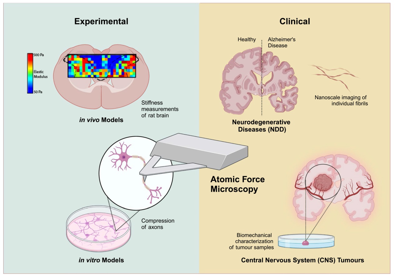
In this review, our aim is to showcase the notable applications of AFM in characterizing experimental models of neurological disorders and to discuss recent advancements in its clinical application for evaluating such disorders. We will provide an overview of the characterization modalities of AFM, and review experimental examples of such application at the molecular, cellular and tissue levels. Additionally, we will highlight the recent progress in the clinical applications of AFM, particularly in the field of neurodegenerative diseases (NDD) and CNS tumours. We will address the challenges that currently hinder the widespread adoption of AFM in clinical settings and discuss emerging technologies and solutions that are poised to overcome these challenges, thereby facilitating its translation into clinical practice.
AFM characterization techniques
The AFM is a multifunctional tool capable of imaging the topography of biological systems at nanometre resolution under physiological conditions. It offers superior spatial resolution and fast imaging time in comparison with other common neuroimaging technologies, including multi-photon microscopy, electron microscopy, ultrasound, CT (Computed Tomography), fMRI (Functional Magnetic Resonance Imaging), MRI (Magnetic Resonance Imaging), SPECT (single photon emission computed tomography) and PET (Positron Emission Tomography) (Table 1) [8⇓⇓-11]. Additionally, it can be used for quantifying biophysical properties and molecular interactions. A wide range of forces (pN to nN) and stiffness (Pa to GPa) could also be measured [12].

Ultrasound, CT, MRI, SPECT and PET are commonly used in clinical settings while the others are primarily used in cellular or tissue studies
AFM operation
AFM typically uses a sharp tip at the free end of a soft cantilever, which is several micrometres long (Fig. 1A). Various probes, ranging from nanometre-sized sharp tips to micrometre- sized beads, are utilized for mechanical characterization of biological samples. Larger probes average measurements over a larger sample area. While sharp probes are preferred for tracing the sample topography and for measuring forces between the probe and sample with high sensitivity (pN resolution). As the AFM probe scans the sample surface, it causes the tip to deflect due to interaction forces. A laser beam aligned to the back of the cantilever reflects onto a photodiode, which tracks the movement of the cantilever and provides positional data in both normal and lateral directions. The cantilever deflection is converted into force by multiplying it by the spring constant of the cantilever. Piezoelectric elements are employed to facilitate precise movements of either the sample or the cantilever. By combining cantilever deflection with XYZ positions, both qualitative data such as morphology and quantitative data including stiffness, hysteresis, adhesion forces can be obtained [12,13].

Fig. 1 a AFM operation principles. AFM utilizes a sharp tip at the free end of a soft cantilever to scan across a sample surface. Height measurements at discrete points create a reconstruction of the sample's topography. b, c Various AFM-based techniques used for characterizing biological samples. Schematics of the force-distance (FD) curves are shown. b The probe indents the sample until it reaches a defined maximum force (blue approach curve) before retracting (black retraction curve) back to its rest position. Stiffness values can be obtained by fitting the slope of the approach curve (a steeper slope corresponds to higher stiffness). The hysteresis or sample viscosity can be estimated from the area between the approach and retraction curves. c The adhesion force (red dot) can be extracted from the retraction curve. Single receptor-ligand interactions can be measured when the AFM tip is functionalized with bioligands |
Morphology
AFM produces topographs with an exceptionally high signalto- noise ratio, allowing direct observation of protein aggregates and fibrils at sub-nanometre resolutions [14⇓-16]. This technique does not necessitate special sample preparations such as surface coating, labelling or dehydration, and it can be used under various conditions (air, and liquid) [17].
AFM operates primarily in two modes: contact and tapping modes [18,19]. Contact mode uses a feedback system to keep the deflection constant, maintaining a constant interaction force between the cantilever tip and the sample. While this mode is quick and sensitive, it can potentially damage soft samples due to the rigid probe making direct contact with the surface. Tapping mode involves the cantilever oscillating near its resonant frequency, controlled by a piezoelectric actuator. A feedback signal maintains a constant amplitude of cantilever vibration during scanning. This mode is preferred in imaging for its ability to achieve high resolution while minimizing damage to the sample. The phase delay between the drive signal and the tip's actual vibration is also measured and used to assess the sample's physical properties.
Besides the usual imaging speeds of few Hz used for imaging static samples, the AFM scanning speed can be increased to observe the dynamic response in biological systems. High-speed AFM (HS-AFM) enables the monitoring of cellular dynamics [11] and the conformational dynamics of single proteins on substrates with sub-seconds temporal resolution. Soft cantilevers (100 - 200 pN/nm) are used for tapping mode imaging to avoid damaging the delicate biological samples. However, using HS-AFM to image the nanostructures of live mammalian cells with length scale of orders of magnitude larger than that of proteins remains complicated [11,13].
Elastic properties
In the force spectroscopy mode, the AFM probe functions as a force sensor to measure the biophysical properties of samples. Stiffness, which denotes resistance to deformations induced by mechanical forces, can be obtained using this mode. The AFM probe indents a compliant sample, such as a cell [20] or tissue [21⇓-23]. The applied force and distance travelled by the probe are recorded in a FD curve (Fig. 1B, C). These FD curves measure the mechanical deformation and response of the sample under load. The approach curve (Fig. 1B) is typically fitted to a Hertz's contact mechanics model, incorporating Sneddon's modification to the indenter shape (for cell/ tissue mechanics). Based on this model, only elastic contributions (Young's modulus) to the sample mechanics are obtained. Besides the Hertz's model, Ogden hyper-elastic material model has also been used for deriving the Young's modulus of brain tissues [23,24]. To conduct accurate elasticity measurements, indentations are generally limited to less than 10% of the sample thickness and regions thinner than 300 nm are avoided as they are likely affected by the underlying substrate [20]. In order to address the heterogeneity of biological systems, an elasticity map consisting of one indent per pixel is usually taken at a region of interest on the sample with the values averaged. Topographs of the region are also generated simultaneously.
The elasticity of mammalian cells, often expressed in terms of the Young's modulus E, is influenced by factors such as cell shape, membrane tension, and cellular compartments. These properties are dynamic and can change during the cell cycle, in response to mechanical stimuli, or due to biochemical signalling [25]. These mechanical properties can undergo significant changes during cell development and in various disease states.
Viscoelastic properties
In complex biological systems (living cells or tissues), they often exhibit time-dependent behaviours (viscoelastic), which manifest as hysteresis between the approach and retraction FD curves (Fig. 1B) [26]. Energy dissipation is the amount of mechanical energy lost as heat during each indentation cycle by the AFM tip, and corresponds to the area enclosed by the approach and retraction curves (areas within the hysteresis loop) [27⇓-29]. This loss of energy is primarily attributed to frictional and viscous damping within the cell or tissue. A larger hysteresis area corresponds to a higher viscoelastic contribution.
Additional techniques for measuring the viscoelastic properties include time domain (static) experiments and frequency domain (dynamic) experiments [23,30]. In time domain experiments, a hold phase is introduced after the AFM tip approaches the sample and before tip retraction. During this hold phase, either the force or deformation is kept constant, while the time-dependent behaviour of the other parameter is measured. Under constant applied force, the deformation is recorded during creep relaxation. Alternatively, stress relaxation can be measured when the deformation is kept constant, while the continuous decay in the interaction force is recorded. In frequency domain experiments, the AFM cantilever oscillates relative to the sample with a small fixed amplitude at a range of frequencies during indentation. The frequency-dependent Young's modulus can be obtained in the context of linear viscoelasticity.
Molecular interaction
AFM is a highly versatile platform for investigating cellular interactions. In addition to probing whole cells, single molecule-based force spectroscopy can be utilized [19,25] to detect the binding strength of ligand-receptor pairs. This technique involves tethering a receptor or ligand to the AFM tip and the cognate ligand or receptor to a substrate. As the tip approaches the substrate, a ligand-receptor bond forms (specific molecular interactions), and subsequent retraction of the tip leads to bond rupture (Fig. 1C). The receptor-ligand bond strength can be inferred from the rupture forces recorded in the forcedistance curve. Specific molecular forces typically range from a few piconewtons and localized receptors on cells can also be simultaneously detected with a lateral resolution of ~ 50 - 100 nm based on the size of the probed molecules and cellular topography [25]. These broad functionalities of AFM underscore its efficacy and applicability in neurobiological research.
AFM characterization of neurological disorders using experimental models
AFM has been used extensively in the study of neurological disorders in experimental models. Selected studies on the biophysical properties characterization at molecular (mapping proteins on neuronal cell membranes) [31⇓-33], cellular (neuronal cells biomechanics) [20,23] and tissue (brain tissue mechanics) [21,22,34] levels are summarized below.
The spatial distribution of ion channels plays a crucial role in neuronal excitability. Maciaszek et al. [31] utilized AFM to detect binding events occurring between specific small conductance calcium activated potassium (SK) channels on the neuron cell surface (cultured hippocampal pyramidal neurons) and apamin molecules (naturally derived bee venom toxins attached to the AFM tip). The SK channels were shown to be highly concentrated on neuronal dendrites membranes, either individually or in pairs. This approach addresses challenges associated with visualizing ion channels at the single-channel level using fluorescent dyes.
Angelman syndrome (AS) is a neurodevelopmental disorder marked by intellectual disability, developmental delays and seizures. There is an accumulation of AS relevant substrate proteins caused by a loss-of-function mutation in the ubiquitin protein ligase E3A (UBE3A) gene. Sun and Yuan et al. [32] investigated the functional properties of 2D human neurons and 3D cortical organoids derived from UBE3A knockout (KO) human embryonic stem cells (hESCs). The loss of UBE3A in human neurons was linked to altered neuronal excitability evidenced by enhanced fast components of after-hyperpolarization (fAHPs) which are regulated by calcium- and voltage-dependent big potassium (BK) channels. BK currents were found to be larger in UBE3A KO neurons compared to wild-type neurons due to increased expression of BK proteins, as confirmed by Western blot analysis. AFM was used to quantify the density of BK proteins on neuron membranes by analysing the interactions between BK proteins on the soma membranes and BK-channel specific antibodies (APC151, Alomone) attached to a functionalized AFM tip (Fig. 2A and B). Results showed a higher density of BK channels in the membranes of KO cells (Figs. 2E and F). Combining these findings with patch-clamp results, BK channels were established to be substrates for UBE3A. As such, targeting BK channels may be viable therapeutic strategy for treating AS.

Fig. 2 Schematics illustrating AFM-based BK probing [32] a Schematic showing the functionalization of the AFM tip with a BK antibody. b Schematics showing the functionalized probe detecting BK channels and FD curves obtained in the presence and absence of BK channels. CM denotes cell membrane. c Representative force-distance curves observed under the various conditions. d Microscopy image and schematic showing the use of an AFM to detect BK channels on neurons using a functionalized probe. e Representative AFM heatmaps displaying specific BK probe binding events over 1 μm2 areas. Colours represent the measured force of specific binding events. f Graphs comparing the unbinding force and BK channel density between WT and KO neurons |
In a recent study by Lim et al. [33], dendron modified AFM probes were used to provide spacing between tethered molecules, thereby improving the probabilities of singlemolecule binding. LIM kinase 1 (LIMK1), a protein involved in the growth of neurons (dendritic spines) was used as a model target protein. By using AFM probes tethered with LIMK1 antibodies, the study analysed LIMK1's distribution within hippocampal neuronal cells, specifically in the soma and dendritic spine areas. In both immature and mature spines, high-resolution force mapping indicated a higher concentration of LIMK1 proteins at the head compared to the shaft, illustrating its vital role in spine development.
In the study by Magdesian et al. [20], the resistance of single axons to damage was assessed through the creation of nanoscale nerve constriction injuries. Axonal degeneration following traumatic brain injury or nerve compression caused by extraneural tissue expansion is a common cause of temporary and permanent disability. Utilizing AFM as both an imaging and mechanical tool, the study compressed axons from rat hippocampal or dorsal root ganglion (DRG) neurons, revealing that DRG axons were significantly more elastic and are at least six times more resistant to mechanical force than hippocampal axons (Fig. 3). Additionally, the elastic modulus (EM) of live axons was measured to confirm that the differential susceptibility of hippocampal and DRG axons to mechanical injury is influenced by differences in elasticity stemming from distinct cytoskeletal architectures. The main components of the axonal cytoskeleton undergo changes during development and myelination. Demyelination, a common occurrence in different degenerative diseases (such as multiple sclerosis or Leukodystrophies in the CNS, and Guillain-Barre syndrome or Charcot-Marie-Tooth disease in the Parasympathetic nervous system (PNS)), was shown to increase neurofilament density, decrease microtubules density, and impede axonal transport in both the PNS and CNS. These alterations in cytoskeletal composition affect the viscoelastic properties of axons and contribute to either increased or decreased axonal resistance to damage. The current model developed for single local degeneration of axons could potentially be applied to drug screening in the field of regenerative medicine.

Fig. 3 Axonal compression experimental model [20]. a (i) A bead attached to the tip of the AFM cantilever was used to gradually compress (sub-nN force) the DRG and hippocampal axons cultured in parallel channels. The axonal response to compression was influenced by the duration and magnitude of the applied force. After releasing the compression force, the four responses include : (ii) axons recovered to the original state, (iii) axons remained permanently deformed, (iv) axons entered a degenerative process characterized by increased focal axonal swelling (FAS), and (v) in severe cases, axonal rupture occurred. DRG axons are more resistant to compression than hippocampal axons. b After compression with 540 Pa for 10 min, DRG axons completely recovered. However, at higher pressures, FAS was resulted along the whole axon (arrows). c Single hippocampal axons were compressed with pressures ranging from 65 - 550 Pa for 10 - 30 mins. Axonal shape and mitochondria transport were not recovered after compression with pressures > 65 Pa for 10 mins. Each panel represents one axon at different time points, before (*), during, and after compression (**). Lower panels denotes 3x zoom of the compression region of the axons before and after compression release. Scale bar : 10 μm |
In a more recent study, Chuang et al. [23] explored the connection between axonal viscoelasticity, fibre anisotropy, and myelination during brain development. Utilizing AFM in conjunction with in situ fluorescent imaging of primary neuron-oligodendrocyte co-cultures from Sprague Dawley rats, they monitored the progressive myelination of axons, noting a corresponding increase in stiffness. By quantifying myelin deposition along axons through immunofluorescence, they established a positive correlation between myelination and increased axonal stiffness over time. AFM measurements indicated that myelinated sections of a single axon consistently exhibited higher Young's modulus values compared to adjacent unmyelinated sections. Furthermore, force-relaxation analysis revealed that the myelin sheath regulates the viscoelastic properties of axons over time. These results underscore a direct link between myelination, axonal orientation, and viscoelasticity, providing crucial insights into the mechanical properties of the developing brain and their relevance to pediatric neurological disorders and injuries.
In order to understand the influence of the mechanical environment on neuronal growth, Koser et al. [22] used the model of developing Xenopus laevis optic pathway to study axon pathfinding. They cultured retinal ganglion cell (RGC) axons on polyacrylamide substrates of controlled stiffness mimicking those of brain tissue (0.1 kPa and 1 kPa). It was found that tissue stiffness regulates axon length and degree of spreading, with axons growing faster and more uniformly on stiffer substrates, while exhibiting slower, more exploratory growth on softer substrates. To further assess the in vivo mechanical environment encountered by RGC axons, AFM was employed to measure stiffness gradients in the developing brain. Tissue heterogeneities were observed at the two different developmental time points and RGC axons were observed to grow perpendicular to the local stiffness gradient in the brain, turning away from stiffer and toward
the softer regions (Fig. 4). Additionally, applying a sustained compressive force of 30 nN with AFM to Xenopus brain, induced local stiffening of the tissue without changing the chemical environment. Similarly, this led to axons avoid growing under the probe where compressive strain was largest. This behaviour highlights the axons' capacity to respond to mechanical cues, a process found to be dependent on the mechanosensitive protein Piezo1. This study emphasizes the critical role of mechanical cues in guiding axonal growth and CNS development.

Fig. 4 Neurons grow toward soft tissue [22]. a Schematic depicting how local gradients in brain tissue stiffness perpendicular to the RGC axon growth direction (M) and the local optic tract (OT) curvature (C) were determined. b Axons turned toward the softer side of the tissue preferentially in vivo. Data plot showing relationship between M and C. c Same data as (B) represented in a bar chat. n : number of measurements from 7 animals. d-e Time-lapse imaging of individual axon bundles growing on a stiffness gradient that mimicked in vivo conditions revealed that in vitro, in the absence of chemical gradients, RGC axons preferentially turned toward the softer side of the substrate. Scale bar : 20 μm. f Eye primordium cultured on a similar stiffness gradient (colour) showed that axons grow more clockwise in the left half and more counterclockwise in the right half of the image, demonstrating a preference for turning toward the softer side of the substrate. Scale bar : 200 μm. g Quantification of individual axon segment orientations confirmed preferential turning toward the soft side of the substrate |
In a study focused on 3D extracellular matrix environments, Ong et al. [21] developed a biomimetic fibre platform to examine how oligodendrocytes (OLs) respond to mechanotransduction during myelination. These fibres, designed to mimic neuronal axons, were fabricated using electrospinning techniques and suspended between supports to establish a stiffness gradient without changing the fibre's topography or diameter. AFM was used to measure the intrinsic stiffness of individual fibres and the overall stiffness of the fibre platform, enabling precise tuning of mechanical properties. On these electrospun fibres, which emulate the diameter of CNS axons, OLs were observed forming myelin sheaths of physiological length. Differentiation was assessed at day 3 by examining the expression of myelin basic protein (MBP) in cell bodies, and myelination at day 10 by confirming the presence of sheaths completely surrounding the fibers. Results showed that increased fibre stiffness led to more cells expressing MBP but fewer cells forming myelin sheaths, suggesting that higher ECM stiffness, as observed in chronic multiple sclerosis (MS) lesions, could hinder remyelination. The study also indicated that OL maturation phases (differentiation and myelination) are regulated independently.
In another investigation, Moeendarbary, Weber and Sheridan et al. [34], assessed the elasticity of healthy rat brain tissue and the changes following a neocortex stab injury using AFM. Glial cells, crucial in local immune responses and wound healing in the CNS, form glial scars post-injury. AFM stiffness mapping of the scarred regions revealed that CNS tissue tends to soften significantly around the injury site, extending outward to distant areas. This softening correlates with increased levels of vimentin, glial fibrillary acidic protein (GFAP), laminin, and collagen IV. Increased vimentin levels, indicates the proliferation of immature glia and new-born neural stem cells. Upregulation of collagen IV and laminin could be a consequence of the destruction of blood vessels. Notably, the largest reductions in cortical elasticity were noted closest to the injury, where upregulation of glial intermediate filaments and ECM components was most pronounced. This softening may hinder neuronal regrowth in adult mammals due to altered mechanical signals, such as those caused by myelin breakdown which exposes inhibitory molecules like Nogo. The study highlighted the soft mechanical signature of glial scars following traumatic injuries, suggesting the need for appropriate mechanical signals in regenerative medicine strategies and neural implant designs to support recovery post-CNS injuries.
Emerging clinical applications of AFM in neurological disorders
Harnessed with the knowledge developed through experimental models and better understanding of the biophysical data, the use of AFM in studying NDD in clinical applications has emerged. Subsequent sections highlight some of the major developments in the study of Alzheimer's Disease (AD), Parkinson's Disease (PD), amyotrophic lateral sclerosis (ALS) and CNS tumours.
Neurodegenerative diseases
NDD are increasingly becoming a societal burden, underscoring the urgent need for better diagnostic and therapeutic strategies. As discussed in previous sections, AFM has emerged as a powerful tool, contributing significantly to our understanding and characterization of the pathogenic mechanisms of neurological disorders in experimental models. Consequently, there is a growing interest in integrating this sophisticated technology into clinical research and the diagnosis of NDD. Current research in this field is hampered by several challenges, including limited therapeutic options and the absence of effective means for early diagnosis, which is crucial for timely intervention [35]. Additionally, there is a lack of disease-specific biomarkers and an incomplete understanding of how misfolded proteins and protein aggregates cause neurotoxicity, which are central to proteinopathic NDDs like AD and PD. In this subsection, we will delve into the clinical applications of AFM in characterizing biomarkers in biofluids such as CSF and blood. We will explore how AFM facilitates nanoscopic structural analysis of these biomarkers, providing deeper insights into the onset and progression of NDD. Furthermore, we will examine recent efforts to enhance AFM's performance in terms of data analysis and quantification, aiming to boost its translational potential for clinical use and diagnosis.
Alzheimer's disease
The current approach to diagnosing AD primarily depends on neuropsychological tests and neuroimaging. However, this method faces significant challenges. The accuracy of cognitive assessments in predicting future risk of progression to AD is often limited, making it difficult to reliably identify the condition at a very early stage [36]. Additionally, the high cost of neuroimaging can be a barrier, leading to situations where individuals receive a late diagnosis or, in some cases, no diagnosis at all [37]. This situation highlights the need for more accessible and accurate diagnostic methods for AD, especially at the pre-clinical stage, where early screening and diagnosis may reduce the risk of developing AD by as much as one third [38].
In this context, CSF has become increasingly important in the clinical assessment of AD [39]. Its interaction with the extracellular regions of the brain mirrors neuropathological changes, making CSF a valuable source for identifying AD biomarkers [40]. However, traditional CSF analysis methods, such as fluorescence correlation spectroscopy [41], are limited due to their reliance on fluorophore labels, which can alter oligomer size distribution [42]. Cryo-electron microscopy has been effective in revealing polymorphisms in brainderived amyloid fibrils [43], but its cryogenic sample preparation process, can potentially distort the fibril structure, thereby affecting the accuracy and usability of the results [44]. As such, AFM has emerged as a useful and promising label-free technique to examine and characterise the protein aggregates in CSF. The insights gained from AFM can potentially revolutionize the diagnosis and prognosis of AD, offering a more precise and reliable approach to understanding this complex condition.
In an earlier effort to resolve the amyloid fibrils in the CSF of patients with mild cognitive impairment (MCI) and AD, Yue and colleagues performed an AFM-based nanoscale characterization of the physical biomarkers in CSF (Table 2), and developed a computational algorithm which integrate these biomarkers and cognitive assessment data to provide an unbiased diagnosis of AD and predict its progression [14]. A subsequent study by De et al. also tapped on the nanoscale sensitivity of AFM and noted higher proportions of larger and longer protofibrilar aggregates in the CSF of AD patients, suggests an important correlation between the size distribution of these aggregates and the progression of disease [15]. A more recent AFM study further confirmed that fibril lengths are higher in CSF of AD patients (Fig. 5A-F) [45]. The fibril length was noted to be inversely correlated with CSF amyloid beta (Aβ) 42/40 ratio and CSF p-tau protein levels, which allows for prediction of amyloid and tau pathology at accuracies of 94% and 82%, respectively.
Table 2 Notable applications of AFM in the evaluation of clinical samples from NDD patients |
 |

Fig. 5 Evaluation of Clinical Samples of NDD Patients Using AFM (a) Schematics of the collection of CSF and the subsequent deposition of protein fibrils on gold substrate within a liquid cell for AFM imaging. b Phase-contrast AFM image showing three distinct conformation of protein fibrillar aggregates in either parallel (green), sliced (red) or T-junction (blue). c-e High resolution AFM height, phase and overlayed images of individual fibrils detected in the CSF of AD patient. f AFM height image of ultralong single fibrils. Adapted and modified from [45]. g The statistical plot, overlayed with a Lorentzian fit, of the mean height of spherical aggregate (red) and the mean height of fibrillar aggregate (grey) on the Red blood cellf (RBC) surface (right insert). h A schematic showing the protein aggregate assembly on RBCs as a function of increasing patient age and decreasing cognition. Adapted and modified from [16]. i-j Representative AFM images of serum from PD patient and healthy control showing extensive presence of aggregates in PD serum. Adapted and modified from [53]. k-n Representative AFM images of platelets from healthy individual (k) and patients with PD (l), ALS (m) and AD (n). Adapted and modified from [55] |
Although AFM is increasingly recognized as a valuable tool for screening AD biomarkers in cerebrospinal fluid, the approach faces fundamental challenges, such as the invasiveness of the lumbar puncture procedure required to obtain CSF. Moreover, it has been observed that amyloid levels in CSF may decrease due to the lumbar puncture itself [46]. As such, blood plasma has emerged as a less invasive alternative for screening [47,48]. However, the presence of numerous non-AD related proteins and biomarkers in the plasma can potentially compromise the efficiency and accuracy of blood-based AD diagnosis [49]. While there are ongoing efforts to evaluate the diagnostic accuracy of blood-based screening of AD biomarkers, there is growing evidence of pathological AD protein aggregates adsorbed on the surface of red blood cells (RBCs). A ground breaking study by Nirmalraj and colleagues performed nanoscopic profiling of protein aggregates on RBCs of AD patients and noted significant age and stage-specific differences in size, shape, morphology, assembly and prevalence of these aggregates (Fig. 5H) [16]. Similarly, Taneva and colleagues also reported significant shrinkage of platelet volume accompanied by 1.5 times higher RBC volume in AD patients [50].
Parkinson's disease
Similar to AD, protein aggregation is also a key factor in the pathogenesis of PD. Dysregulated protein homeostasis leads to the accumulation and aggregation of neurotoxic proteins such as β-amyloid and α-synuclein [51]. These aggregates spread and accumulate further, overwhelming the clearance systems and ultimately resulting in neuronal death [52]. However, little is known about the characteristics and distribution of the subspecies of these oligomeric proteins. They exist in low concentration down to sub-picomolar level, and highly heterogenous in terms of size and structure, posing significant challenges for current measurement and quantification methods. As such, Labonova and colleagues harnessed the high resolving capability of AFM to analyse both the serum and CSF from PD patients (Fig. 5I and J) [53]. Their research revealed a higher proportion of protein aggregates exceeding 150 nm in length in PD patients. Moreover, they observed a distinct distribution of β-sheet aggregates between PD patients (50% α-synuclein and 50% β-amyloid) and control subjects (30% α-synuclein and 70% β-amyloid). This specific ratio enabled the discrimination of PD cases from controls with an impressive accuracy of 98.2%. These findings, made possible by the nanoscopic resolution of AFM, hold significant promise for future applications in diagnostics, monitoring PD progression, and evaluating the efficacy of PD therapies.
Additionally, several AFM studies focusing on blood cells in PD patients showed trends similar to those in AD patients. Strijkova-Kenderova and colleagues noted distinct differences in shape, size and volume of RBCs in PD patients, where the RBCs are predominantly exhibited a crenate shape, and significantly larger in terms of diameter and volume as compared to RBCs from healthy subjects [54]. Following this, Taneva and colleagues conducted a study that reported a significant shrinkage in platelet volume by 55.7% and a 1.5-fold increase in RBC volume compared to healthy controls. Furthermore, this study highlighted a notable reduction in the surface roughness of RBCs in PD patients, indicating a substantial membrane smoothening due to modified cytoskeletal integrity. Complementing these findings, Strijkova and colleagues performed a separate study on platelets from PD patients and reported similar cellular properties, as shown in Fig. 5K-N and outlined in Table 2, along with marked increase in the platelet stiffness when compared to healthy subjects [55]. These studies collectively offer valuable insights into the cellular alterations in PD, enhancing our understanding of the disease at a nanoscopic level.
Amyotrophic lateral sclerosis
Despite being one of the most common and degenerative motor neuron disease, ALS still lacks clinically validated, reliable and specific markers for diagnosis and progression monitoring [56]. There are ongoing efforts to identify new biomarkers and validate the growing list of potential biomarkers in CSF, including TAR DNA-binding protein 43 (TDP-43) [57], neurofilament light chain (NfL) [58] and mutations in superoxide dismutase 1 (SOD1) gene [59]. Interestingly, there are emerging indications that Aβ42 might play a role in ALS pathogenesis [60,61]. The study by Colletti and colleagues found that ALS patients with a lower Aβ42/40 ratio had a shorter survival period, although neither the level of Aβ 1-42 nor the Aβ42/40 ratios influenced the rate of disease progression [60].
This lack of correlation may be better understood through insights from AFM-based studies on the CSF samples from AD patients. These studies suggest that rather than the types of protein aggregates, specific subspecies of protein aggregates and fibrils, defined by their length, size and conformation, might be more neurotoxic and contribute to disease onset and progression. Traditional detection methods, such as ELISA-based antibody capture of the proteins, lacks the nanoscale resolving power of AFM and often only provide data on the total mass of aggregates. This approach potentially overlooks crucial details about the subspecies of protein aggregates, including size and length, which may play a pivotal role in the pathogenesis of neurodegenerative diseases like AD and ALS.
Building on the need for more precise antibody enrichment tools in neurodegenerative disease research, Williams and colleagues developed a novel AFM-based biopanning technique specifically designed to isolate antibodies based on their morphology [62]. These antibodies are highly selective for specific protein variants of TDP-43, which are exclusively found in human ALS brain tissue. By tapping on the unique capabilities of AFM, the team performed multiple rounds of negative panning steps to remove phage clones that bound to off-target antigens, further enriching the pool of clones specific to target protein variants during the positive panning step. This technique represents a significant advancement, offering a more targeted method for identifying and studying protein variants associated with ALS.
Central nervous system tumours
The Central Nervous System (CNS) consists of the brain and spinal cord, functioning as the central processing hub for the entire body. It orchestrates a wide array of complex functions, from regulating involuntary processes like breathing to enabling conscious movement, sensory experiences, and cognitive functions [63]. The neuropathological classification of CNS tumours, such as glioblastoma multiforme (GBM) and meningioma, primarily relies on the grading system published by World Health Organization (WHO), which largely depends on microscopy-derived histomorphological features [64]. However, this grading system faces significant intra- and inter-observer variability arising from the complexity of morphological details which varies extensively across different tumours and patients. Additionally, the system is further complicated by technical variations in histopathological procedures like staining protocols. The individual experience of the diagnosing pathologist also plays a vital role, as different levels of expertise can lead to varied interpretations of the same histological features, resulting in the diagnostic variability of the grading system [65].
Accurate grading of brain tumours is crucial because it not only determines the patient's prognosis but also dictates the choice of treatment options. In pursuit of enhancing the assessment and grading of CNS tumours, clinicians are now incorporating biophysical methods like AFM into the process, which provides nanometre resolution and offers a more detailed analysis of tumour properties using freshly resected tumour tissues. This integrative approach facilitates a more precise and comprehensive evaluation of CNS tumours, which is essential not only for effective patient management, but may also improve current surgical practice and potentially leading to more complete tumour excision. In this subsection, we will explore recent AFM-based studies on CNS tumour stiffness and how these findings may be useful in clinical practice. We will also examine how complementary experimental modalities to AFM have provided additional insights and contributed to reducing variability in tumours grading. Finally, we will discuss the translational challenges of AFM in clinical diagnostics and highlight ongoing efforts to address these shortcomings.
In their pioneering study, Ciasca and colleagues used AFM to study the nano-mechanical properties of freshly resected human GBM and meningioma tissues. They reported significant difference between the stiffness of GBM tissues and the adjacent normal peritumour regions, with tumour tissue being up to 10 times stiffer than normal tissues [66]. Furthermore, the team was able to establish a Young's modulus maps of GBM tumours, revealing that non-necrotic tissues exhibited distinct peaks corresponding to soft and stiff structures, while necrotic tissues displayed a more uniform distribution. These findings potentially offer unique biomechanical signatures that could assist in the classification of GBM progression. These observations align with the work by Ciesluk and colleagues, who noted not only a higher stiffness in GBM tissues, but also a pronounced heterogeneity within the primary gliomas and the resultant metastatic tumours [67]. The stark contrast in stiffness, together with additional information such as stiffness distribution mapping of the tumour sample, has great potential for enhancing surgical practice, particularly in redefining the extent of tumour excision, which may lead to improved surgical outcomes and better patient prognosis.
Furthermore, the current grading system for CNS tumours could be enhanced by incorporating nanomechanical properties, as emerging evidence suggests that tumour stiffness, sometimes manifesting before obvious histological and clinical signs, may affect growth and metastatic potential [68,69]. While the relevance of mechanical parameters is clear, it's also crucial to understand the biochemical underpinnings of these nanomechanical differences, as they offer significant insights into neuropathological processes. In this context, Abramcyk and Imiela have pioneered work by using AFM for stiffness evaluation of fresh brain tumour tissues and complemented this with Raman spectroscopy and imaging to analyse the biochemical composition [70]. They noted significant dysregulation of protein and lipid metabolism in malignant medulloblastomas, associated with elevated stiffness and heterogeneity. These biochemical and nanomechanical signatures could be key in the identification of predictive cancer markers and evaluation of treatment options that target the mechanical aspects of cancer progression.
Despite the growing recognition of AFM-derived stiffness data in evaluating CNS tumours, there are inherent challenges and technical limitations in the traditional histomorphological workflow that contribute to observer variability in the current grading system. Unlike conventional histological methods, AFM requires no staining, thereby avoiding complications that may arise from factors like section thickness, fixation time, and the types or purity of reagents which all may contribute to variations in results. Consequently, the topographical data generated from AFM scans offer a more robust and objective approach in the neuropathological assessments of CNS tumours samples. Furthermore, even with consistent histomorphological data, grading accuracy can be affected by varied assessments from individual observers, influenced by differences in experience and interpretation of morphological information. Addressing this issue, Schilcher's research group adopted a data-modelling and genetic programming approach to classify AFM images of CNS tumours and attained accuracy of over 90% [71,72]. This computer-assisted approach was designed to minimizes the intra- and inter-observer variations in tumour grading, and has demonstrated a 94.74% accuracy in distinguishing grade II tumours that were previously classified as grade IV, thereby enabling a more accurate and tailored therapy option [72].
While AFM shows promising potential in providing quantitative insights to the evaluation of surgically removed CNS tumours, there remains a considerable gap in fully implementing this technique in clinical diagnosis. One of the key obstacle of the translational process is the complexity of AFM data analysis, which is both time consuming and requires specialised knowledge in physics and mathematics [73]. To bridge this gap, researchers have developed various automated workflow that significantly enhance the efficiency of data analysis and enable the integration of such data into the classification of tumours. A notable advancement in this area is the development of a fully automated neural network approach by Minelli and colleagues for analysing AFM data of histologically classified tumour samples. This innovative approach, which is both model-free and operator-independent, bypasses the need for FD curve fitting and further interpretation, thus functioning as a direct diagnostic tool [74]. The team reported good classification of the tumour samples, and it appears to be more effective than the conventional FD curve fitting, which only considers a small portion of the FD curve.
A more recent effort from the same research team have explored strategies to reduce the AFM measurement time [75]. They have modelled AFM mapping using a binomial process, based on the estimation of the minimal number of FD curves needed to classify CNS tumour tissue with a 0.005 confidence level. Although the findings are largely preliminary and a more complex and comprehensive models are required to validate the applicability of the approach, its promising results indicate a potential direction for future efforts in enhancing the practicality of AFM in clinical settings. This development represents a significant step towards making AFM a more feasible and effective tool in the clinical evaluation of CNS tumours Table 3.
Table 3 Notable clinical applications of AFM in the evaluation of CNS tumour samples |
 |
Challenges and limitations
In order to provide a more accurate and reliable diagnosis of NDDs using AFM based morphology and mechanics-based markers, the challenges and limitations of AFM (Table 4) should be considered. Some of the possible solutions to mitigate these challenges are presented below.
Table 4 Challenges and limitations of AFM use in clinical applications |
 |
One limitation of AFM is the reliance on manual operation and experience in locating areas of interest such as specific cells within a tissue sample for measurements, resulting in low throughput. Commonly, fluorescence-based techniques are employed to pinpoint these areas. For instance, Fuhs et al., identified differences in mechanical properties between naive and ischemia-affected brain regions by detecting green fluorescence signals from FITC-albumin in mouse brain slices, indicating compromised blood-brain barrier integrity [77]. An alternative approach involves using deep learning-assisted AFM [78], which facilitates fluorescence-independent identification and automated force measurements of cells. This method utilizes deep learning algorithms to recognize cell viability and type from optical bright-field images without labels. It automatically determines the positional relationship between the AFM probe and the targeted cells, enabling precise and efficient probe positioning for high-throughput force measurements. Further advancements in AFM technology, like those introduced by Kang et al. [79], have led to the development of an autonomous AFM capable of automated initialization, surface imaging, and analysis. The system utilizes a faster region-based convolutional neural network (faster R-CNN) algorithm to identify and locate the laser spot, cantilever, and sample surface in space. Using this positional data, the system autonomously calibrates and initializes its components for topographic imaging. Additionally, the same faster R-CNN algorithm was used to detect the objects of interest in acquired images and perform image analysis. This autonomous setup is critical for enhancing operational efficiency and reducing the manual expertise required.
A significant challenge in AFM imaging is the extensive time required to produce high-resolution image maps (> 256 x 256 pixels) of large number of cells or tissue areas. To enhance speed, one strategy is to reduce the number of pixels and scan lines measured. However, this can compromise the resolution of the final images. To counteract this loss of detail, deep learning models like very deep superresolution (VDSR) [80] or a deep neural network can be utilized to reconstruct μ-path pattern sub-sampled AFM images [81]. Another method to increase scanning speed while minimizing sample damage involves using High-Speed AFM (HS-AFM) with an extremely long AFM tip (a 3 μm long, 5 - 8 nm in diameter amorphous carbon grown tip on a 100 - 200 pN/nm soft cantilever). This setup not only achieves high spatial resolution but also reduces the risk of cell damage during fast tapping-mode scanning (~100 nm free amplitude, 800 kHz) [11]. Additionally, a novel technique known as Ringing mode™ (developed by NanoScience Solutions, Inc.) offers a substantial improvement, being up to 20 times faster than traditional sub-resonance tapping modes like Peak Force Tapping, HybriD, and Digital Pulse. This mode also simultaneously records eight new physical parameters of the samples including restored adhesion, adhesion height, disconnection height, pull-off neck height, disconnection distance, disconnection energy loss, dynamic creep phase shift and zero-force height. The Ringing mode™ is based on an analysis of ringing signal (typically regarded as noise and filtered out in the existing modes) of the AFM cantilever which occurs after the AFM probe detaches from the sample surface [83⇓-85]. This innovative approach allows for faster and more detailed AFM imaging with less artifacts.
Interpreting AFM topographs can be challenging, particularly when distinguishing cells or features of interest among similar height features. To address this, a diagnostic approach using discrete Fourier transforms (DFTs) of standard AFM section measurements has been developed to distinguish neural cell edges from their scaffold backgrounds [86]. This method employs a Gaussian and Butterworth frequency domain high-pass (GHPF) filter of appropriate degree and cutoff frequency designed to accentuate the high-frequency harmonics of the tissue scaffold. This enhancement improves the feature definition of nanoscale cellular edges in the images. During AFM imaging, some artifacts or image distortions may obscure the actual surface features. Post-processing often becomes necessary to eliminate or minimize these discrepancies, ensuring clarity and accuracy of the surface images. A convolutional neural network-based method using the ResUNet architecture has been developed to reduce imaging artifacts and noise while maintaining crucial topographical features, such as edges [82]. Analysing AFM images for brain tumour diagnosis in neuropathological brain tissue samples presents significant difficulties due to the intricate nature of these images and the challenge of extracting relevant structural details. A sophisticated approach combining data modelling and genetic programming has been implemented to classify AFM images of central nervous system (CNS) tumours, achieving classification accuracies over 90% [71,72]. This high level of accuracy is crucial for effective diagnosis and enhances the utility of AFM in medical diagnostics.
For AFM mechanical properties measurements, a major obstacle in the use of AFM in clinics is the complexity of the data analysis. It requires specialized, experienced personnel in the processing (curve fitting through mathematical models) and interpretation of data. An innovative solution is the use of neural networks for pattern recognition of FD curves (based on curve shape) to automatically classify them, eliminating the need for curve-fitting with complicated mathematical models [74,75]. Measured FD curves are often disturbed by detachment of samples from supporting substrate, irregularities of the heterogeneous sample surface or large adhesive forces between sample and AFM probe. These artifacts could be spotted by an experienced experimentalist and the data curve discarded before evaluation. However, such methods of manual sorting are time consuming for large datasets. Machine learning can be used to identify artefactual force curves relative to good curves, providing a fast and accurate way to perform automated and operator independent analysis of large datasets [87,88].
To enhance the chemical characterization capabilities of AFM, it can be integrated with other spectroscopic techniques. AFM tips can act as probes for chemical identification in addition to mapping sample topography. AFM-IR (AFM-infrared spectroscopy) [94] combines a pulsed, tuneable infrared laser with an AFM, enabling nanoscale molecular chemical analysis. Similarly, Tip-enhanced Raman spectroscopy (TERS) AFM [92] provides nanoscale chemical and structural information without the use of labels common in super-resolution optical microscopy. These labels could potentially affect the structures of labelled species and their interactions. This technique uses optical coupling to direct an excitation laser to a metallic AFM tip, enhancing the Raman scattering at the tip-sample junction and producing a hyperspectral image with precise chemical contrast.
The combination of AFM with optical spectroscopy, such as with AFM-IR [90,91] and TERS [92,93], are particularly useful for studying proteins associated with neurodegenerative diseases. For example, AFM-IR has been employed to reveal significant structural variations in amyloid oligomers through their infrared spectra [90]. Additionally, tip-enhanced Raman spectroscopy has provided nanoscale chemical mapping of single amyloid fibrils throughout various stages of aggregation, offering valuable insights into the fibril formation process [92]. These enhancements extend the utility of AFM from physical to chemical analysis, broadening its application in medical research and diagnostics.
In addition to challenges like the high cost of equipment and the need for broader clinical acceptance, AFM faces several barriers in clinical adoption. Despite these hurdles, innovative solutions are emerging to address them. Increasingly, the use of morphology and mechanics-based markers is being recognized for their potential in clinical applications [95,96]. Notably, the commercial nanotechnology platform ARTIDIS R (https://artid is.com/) has been developed to offer rapid diagnostic services. This platform can diagnose cancer, assess its aggressiveness, and predict the likelihood of metastasis development in less than three hours, utilizing a nanomechanical biomarker. It employs a nanomechanical sensor to analyse the physical properties of tumour cells and their microenvironment. Integrating this information with clinical data, the platform can identify aggressive types of cancer and customize treatment plans for individual patients, enhancing personalized medicine in oncology.
Conclusions and future perspectives
Neurological disorders are becoming an increasingly significant societal burden, highlighting the critical need for improved diagnostic and therapeutic approaches. As previously discussed, AFM has proven to be a powerful tool, greatly enhancing our understanding of the pathogenic mechanisms of neurological disorders in experimental models. There are also considerable efforts underway to integrate this unique technology into clinical research and the diagnosis of neurological disorders, with the potential to use morphology and mechanics-based markers for identifying various NDDs and CNS tumours.
Despite the significant potential of Atomic Force Microscopy (AFM) in clinical settings, its widespread adoption faces challenges, particularly the time-intensive nature of measurements and the complexity of data analysis. Addressing these limitations, the integration of advanced machine learning techniques, including neural networks for classification and automated analysis of force-distance (FD) curves, alongside optimized spatial sampling, shows promise in overcoming these hurdles while maintaining diagnostic accuracy [75]. Moreover, ongoing advancements in computational modelling and big data analytics are set to further enhance the functionality and efficiency of AFM. These innovations could facilitate the processing of the extensive data generated by AFM, potentially enabling a future where real-time analysis and interpretation could be achieved in scenarios requiring quick diagnostic decisions, such as during acute neurological emergencies or neurosurgical procedures. Furthermore, developments in high-throughput AFM technologies could enable the rapid screening of large patient cohorts, facilitating early diagnosis and the monitoring of disease progression and response to treatment. This capability would be especially crucial in managing neurodegenerative diseases, where early intervention can significantly alter disease trajectories.
Furthermore, with the advent of commercial nanotechnology platforms like ARTIDISR, there is a growing possibility of adopting personalized treatment strategies based on morphology and mechanics-based markers [13,95,96]. These technologies facilitate the tailoring of therapeutic approaches to individual patient profiles, which could revolutionize the management of neurological disorders. The potential for these platforms to make personalized medicine more accessible promises a significant shift in how neurological conditions are treated, potentially leading to better patient outcomes.
Looking forward, the future of AFM in neurology is set for transformative growth. As AFM technology continues to integrate with other imaging modalities and omics technologies, it holds the promise of uncovering novel biomarkers and therapeutic targets, thereby enhancing the precision of diagnostics and treatments. The ongoing evolution of AFM, combined with breakthroughs in computational analysis and broader diagnostic technologies, is poised to make substantial contributions to the field of neurology, not only deepening our understanding of neurological diseases but also improving patient care through more precise and personalized treatment strategies.
Acknowledgements This work was supported by the Institute for Health Innovation and Technology (iHealthtech), MechanoBioEngineering Laboratory at the Department of Biomedical Engineering, the Mechanobiology Institute and the Institute for Functional Intelligent Materials (I-FIM) at the National University of Singapore. The graphical abstract was created with BioRender.com.
Authors' contributions Conceptualization: D.T.S., M.H.N. and C.T.L.; writing - original draft preparation: D.T.S. and M.H.N.; writing - reviewing and editing: D.T.S., M.H.N. and C.T.L. All authors have read and agreed to the final version of the manuscript.
Funding Not applicable.
Availability of data and materials Not applicable.
Declarations
Competing interests C.T.L. is an Associate Editor for Med-X. C.T.L. was not involved in the journal's peer review of, or decisions related to, this manuscript.
Open Access This article is licensed under a Creative Commons Attribution 4.0 International License, which permits use, sharing, adaptation, distribution and reproduction in any medium or format, as long as you give appropriate credit to the original author(s) and the source, provide a link to the Creative Commons licence, and indicate if changes were made. The images or other third party material in this article are included in the article's Creative Commons licence, unless indicated otherwise in a credit line to the material. If material is not included in the article's Creative Commons licence and your intended use is not permitted by statutory regulation or exceeds the permitted use, you will need to obtain permission directly from the copyright holder. To view a copy of this licence, visit http://creativecommons.org/licenses/by/4.0/.
Publisher's Note Springer Nature remains neutral with regard to jurisdictional claims in published maps and institutional affiliations.
